Discrete Fourier Transform For Freuency Analysis
11 Oct 2014Introduction
Fourier analysis is generally concerned with the analysis and synthesis of functions. The decomposition of signal into easy-to-analyze components and the reconstruction from such components.
In this article we will look at Fourier analysis of discrete time signals.
Discrete time signal are defined at only particular set of time instances and are represented as sequence of real numbers that have continuous range of values
Fourier Series Representation of signal
A discrete time complex exponential is periodic in nature
$ e^{j k\omega (n+N)} = e ^{j k \omega n} $ where , $\omega=\frac{2\pi}{N}$
The set of all discrete time time complex exponential signals that are periodic with period N is given by $\phi_{k}[n] = e ^{j k \frac{2\pi}{N} n} , \forall k \in \mathcal{Z}$
\(\phi\_{k+rN}[n] = e ^{j (k+rN) \frac{2\pi}{N} n} = e ^{j k \frac{2\pi}{N} n} * e ^{j r N \frac{2\pi}{N} n}\) \(\phi\_{k+rN}[n] = e ^{j k \frac{2\pi}{N} n} e ^{j r 2\pi n} =e ^{j k \frac{2\pi}{N} n}\)
When k is changed by integral multiples of N ,we get identical sequence. Thus there are only N unique values of k for which we can define unique discrete time complex exponential sequence.
\[\begin{align} x[n]=\sum\_{k} x[k] e^{j k \omega n} \end{align}\]$e^{j k \omega n} $ are only unique over N successive values of k,summation is only considered over this range
\[\begin{align} x[n]=\sum\_{k={N}} x[k] e^{j k \omega n} \end{align}\]$x[n]$ is periodic with period N.
Discrete time Fourier Series
Let us consider a arbitrary periodic signal $x[n]$ with period N and that $x[n]$ can be expressed in the form
\[\begin{align} x[n]=\sum\_{k} X[k] \phi\_{k}[n] \end{align}\]Thus we need to find out if $x[n]$ can be expressed in the above form and if so the coefficients $x[k]$ for which this representation is valid.
The theoretical derivations for the same can be found in all signal processing references.The result are as follows
\(\begin{align} X[k] =\sum\_{n=0}^{N-1}x[n] e^{- j k \frac{2\pi}{ N} n } \end{align}\) and \(\begin{align} x[n] =\frac{1}{N}\sum\_{k=0}^{N-1}X[k]\,e^{j k \frac{2\pi}{ N} n } \end{align}\)
$X[k]$ are called as Fourier series coefficients.The coefficients are also referred to as spectral coefficients of signal $x[n]$.
The representation of signal $x[n]$ in terms of spectral coefficients is called as the Fourier series representation of the signal
These coefficient specify the decomposition of signal $x[n]$ into sum of N harmonically related complex exponential .
Any periodic discrete time signal $x[n]$ can be represented using the Fourier series representation and Fourier series representation enable us to represent any periodic signal as weighted sum of complex exponential s.
Let us look at some examples to understand what information can Fourier series representation of a signal give us.
def FourierSeries(input,N=None):
    """ computes the fourier series coefficients of input signal

    Parameters
    -----------
    input : numpy array
            input discrete time signal

    Returns
    --------
    out : complex,list
          fourier series coefficients
    """

    N=len(input);

    w=2*cmath.pi/N;
    input=input[0:N];
    n=numpy.arange(0,N);
    r=cexp(-1j*w*n);

    output = [complex(0)] * N
    for k in range(N):
        r=input*cexp(-1j*w*n*k)
        output[k]=np.sum(r);


    return output;
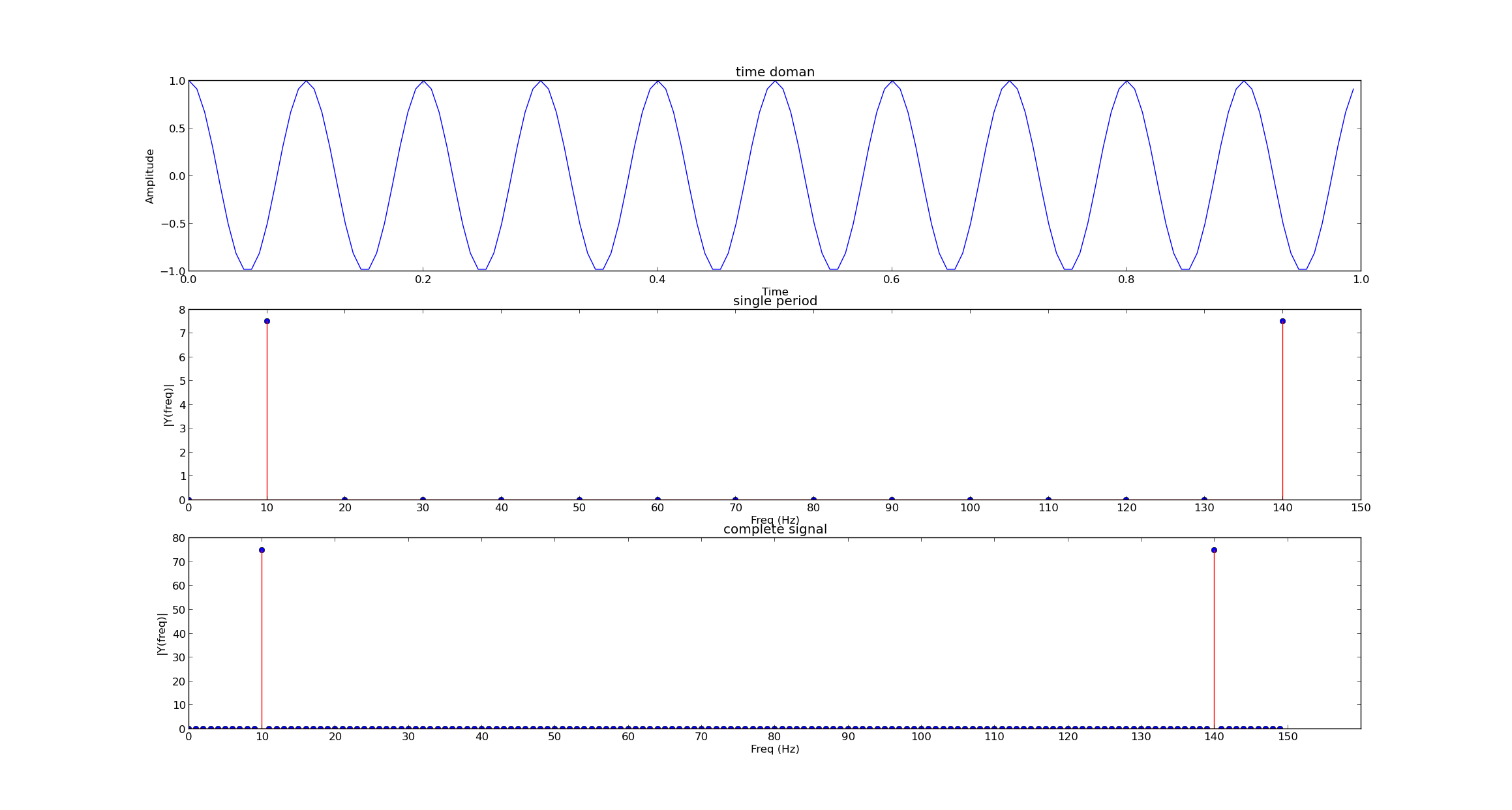
Let us consider a sinusoidal signal with frequency $f_{s}=10Hz$,for a duration of 1sec Lets sample this waveform at $F_{s}=150Hz$ and observe the Fourier series coefficients of the signal
we sample at 150Hz,In the frequency spectrum,just consider a single period of the cosine waveform,ie $F_{s}/f_{s}=15$ samples.The output can be seen in subplot 2
we take complete signal,and compute the Fourier series coefficients,output can be seen in subplot 3
Let us consider magnitude plot of Fourier series
def FourierSinusoids(F,w,Fs,synthesis=None):
    """ the function generates a discrete time sinusoid,computes
	the Fourier series coefficients and plots the time and frequency
	data

     Paraneters
     ----------
     F : numpy array
         sinuoidal frequency components

     w  : numpy array
          the weights associated with freuency components

     Fs : Integer
          sampling frequency

     synthesis : int
                 if 1 ,reconstructs signal and plots the original and reconstructed
                 signal

    """
    if synthesis==None:
        synthesis=0;

    Ts=1.0/Fs;
    xs=numpy.arange(0,1,Ts)

    signal=numpy.zeros(np.shape(xs));
    for i in range(len(F)):
        omega=2*np.pi*F[i];
        signal = signal+ w[i]*numpy.cos(omega*xs);
    #plot the time domain signal
    subplot(2,1,1)
    plt.plot(range(0,len(signal)),signal)
    xlabel('Time')
    ylabel('Amplitude')
    title('time doman')
    #plt.ylim(-2, 2)

    #compute fourier series coefficients
    r1=FourierSeries(signal)
    a1=cabs(r1)

    if synthesis==0:
        #plot the freuency domain signal
        L=len(a1);
        fr=np.arange(0,L);
        subplot(2,1,2)
        plt.stem(fr,a1,'r') # plotting the spectrum
        xlabel('Freq (Hz)')
        ylabel('|Y(freq)|')
        title('complete signal')
        ticks=np.arange(0,L+1,25);
        plt.xticks(ticks,ticks);
        show()

    if synthesis==1:
        rsignal=IFourierSeries(r1);
        print np.allclose(rsignal, signal)
        subplot(2,1,2)
        plt.stem(xs,signal)
        xlabel('Time')
        ylabel('Amplitude')
        title('reconstructed signal')
        show()


if __name__ == "__main__":

    mode =0

    if mode==0:
        F=[10];
        F=np.array(F);
        w=numpy.ones(F.shape);
        #plot the time domain signal and fourier series component
        FourierSinusoids(F,w,150);
we can see that the frequency corresponding to 10Hz we can observe peak.The total number of Fourier series coefficients are equal to the total number of input samples.
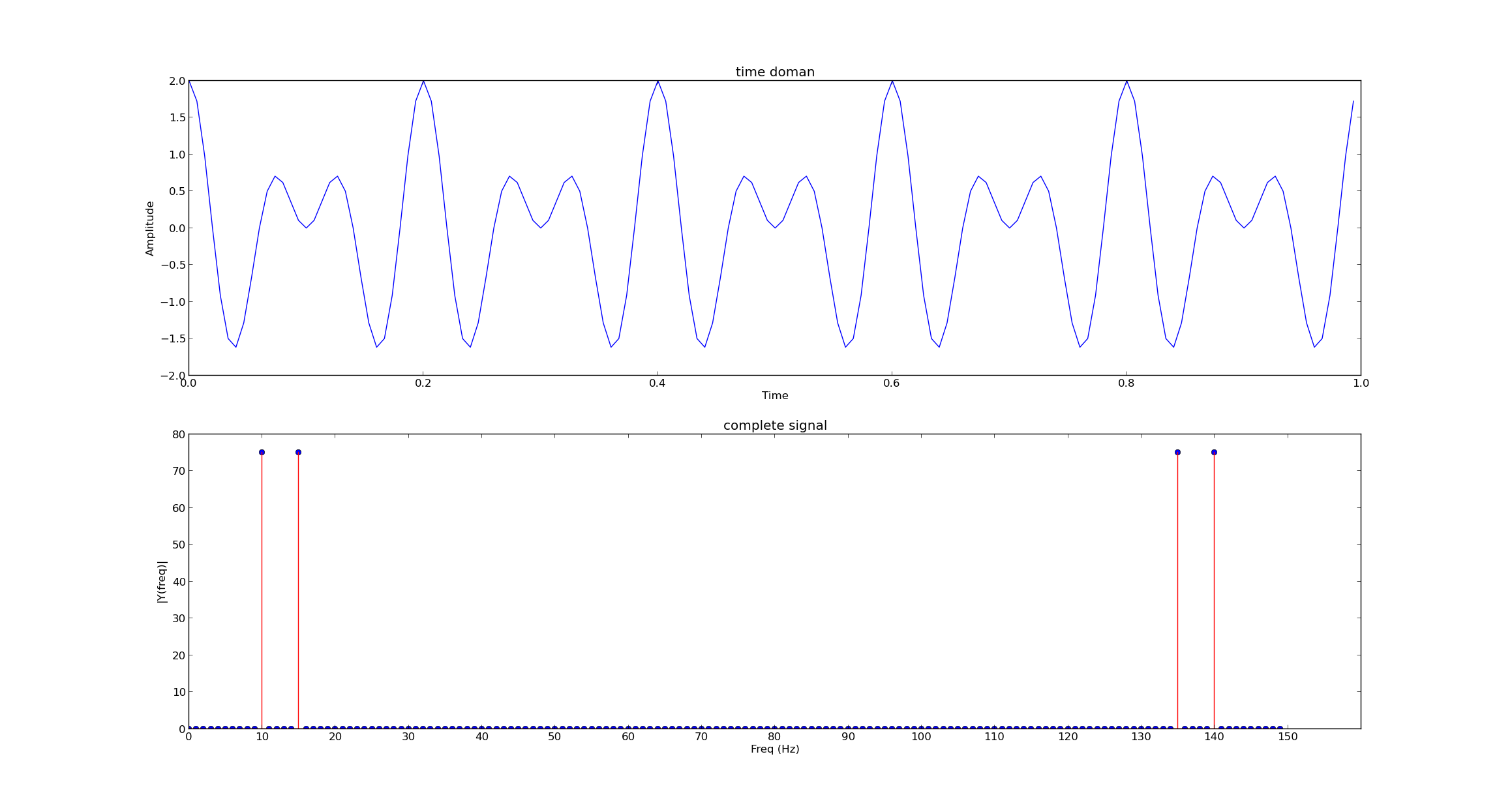
Now let us consider a combination of sinusoidal signals at freuency 10 and 15Hz.The signal is periodic with frequency which is LCM of 10 and 15 ie 5Hz.
    if mode==1:
        F=[10,20];
        F=np.array(F);
        w=numpy.ones(F.shape);
        FourierSinusoids(F,w,150);
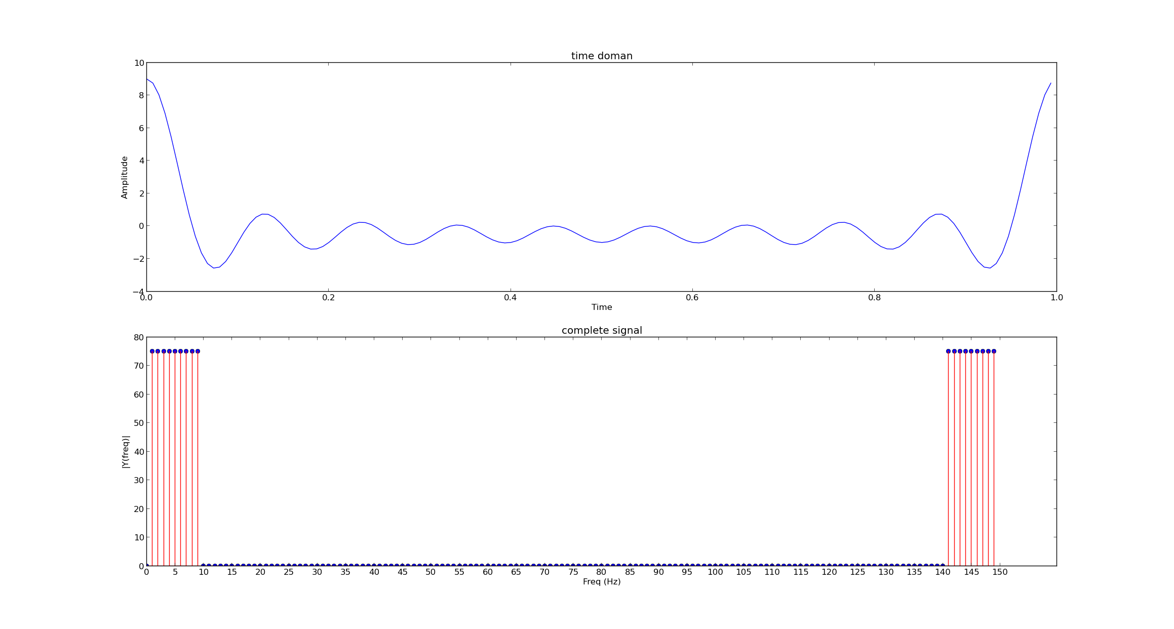
Now lets keep on adding frequency components.The below signal is periodic with period of 1 sec
    if mode==2:
        F=range(1,10);
        F=np.array(F);
        w=numpy.ones(F.shape);
        FourierSinusoids(F,w,150);
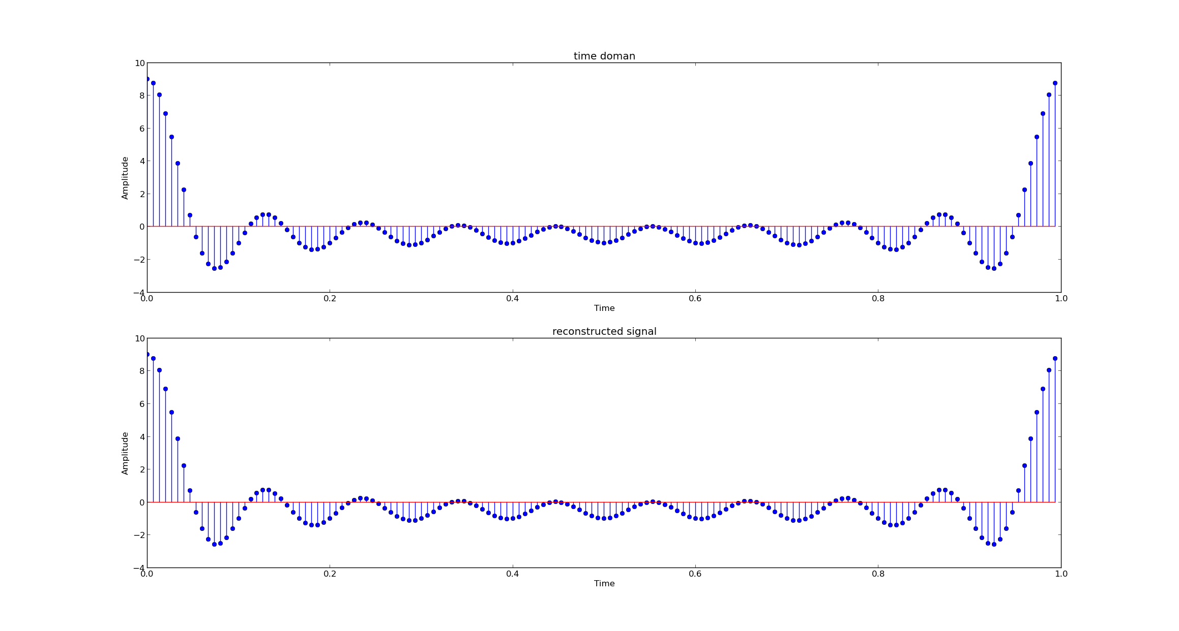
Synthesis of Signal
In the earlier section we saw the process of decomposition of aperiodic signal into its frequency components.
we will now look at the synthesis of signal from its Fourier series coefficients.
\[{x[n] = \frac{1}{N}\sum\_{k=0}^{N-1}X[k]\,e^{j k \frac{2\pi}{ N} n }}\]Below is plot of the original and reconstructed signal and python code for the
def IFourierSeries(input):
    """ function reconstructs the signal from fourier series coefficients

    Parameters
    ---------
    input : cmath list
            fourier series coefficients

    Returns
    -----------
    out : numpy arrary
          reconstructed signal

    """
    N=len(input);
    w=2*cmath.pi/N;
    k=numpy.arange(0,N);
    output = [complex(0)] * N
    for n in range(N):
        r=input*cexp(-1j*w*n*k);
        output[n]=np.mean(r);

    print output.__class__
    return output;


    if mode==3:
        F=range(1,10);
        F=np.array(F);
        w=numpy.ones(F.shape);
        FourierSinusoids(F,w,150,1);
Discrete Fourier Transform
Now arises the situation what do we do for a-periodic signals.After a lot of theorotical analysis on Discrete time Fourier transform and sampling in the frequency domain,it turns out we just assume periodic extension of aperiodic signal and compute Fourier series as above.
The Fourier series coefficients for a periodic signal are also periodic with same period N
\[X[k+N]=X[k]\]If we consider a single period of N values of Fourier series coefficient ,we obtain a finite duration sequence which is called Discrete Fourier Transform (DFT).
Thus by computing the DFT we obtain the Fourier series coefficients for single period.
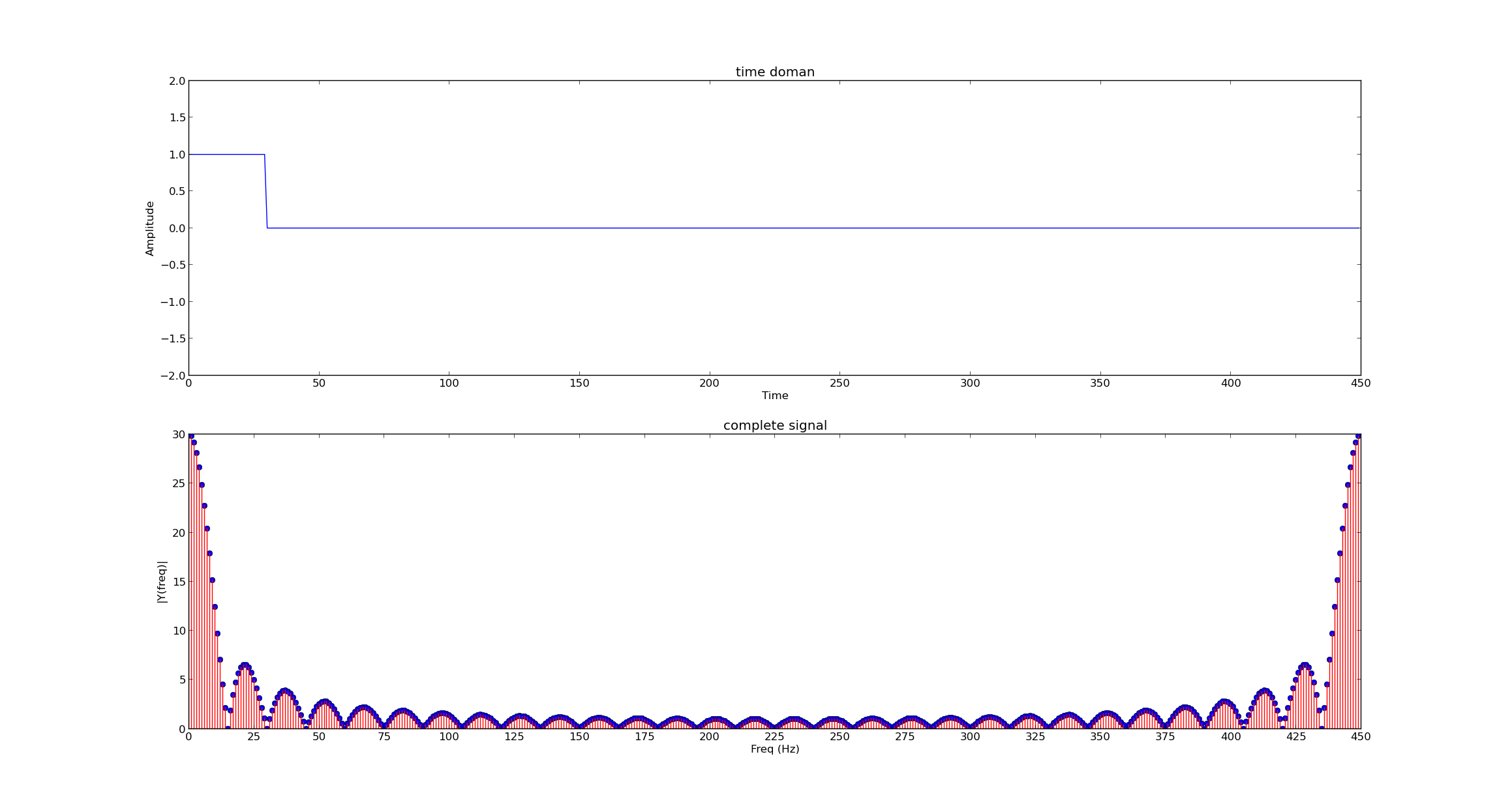
It is upto us to choose a period of the signal.Let us consider a aperiodic impulse of length 150 and on-duty cycle of 5.
Let us consider N=150,450 and observe the results.
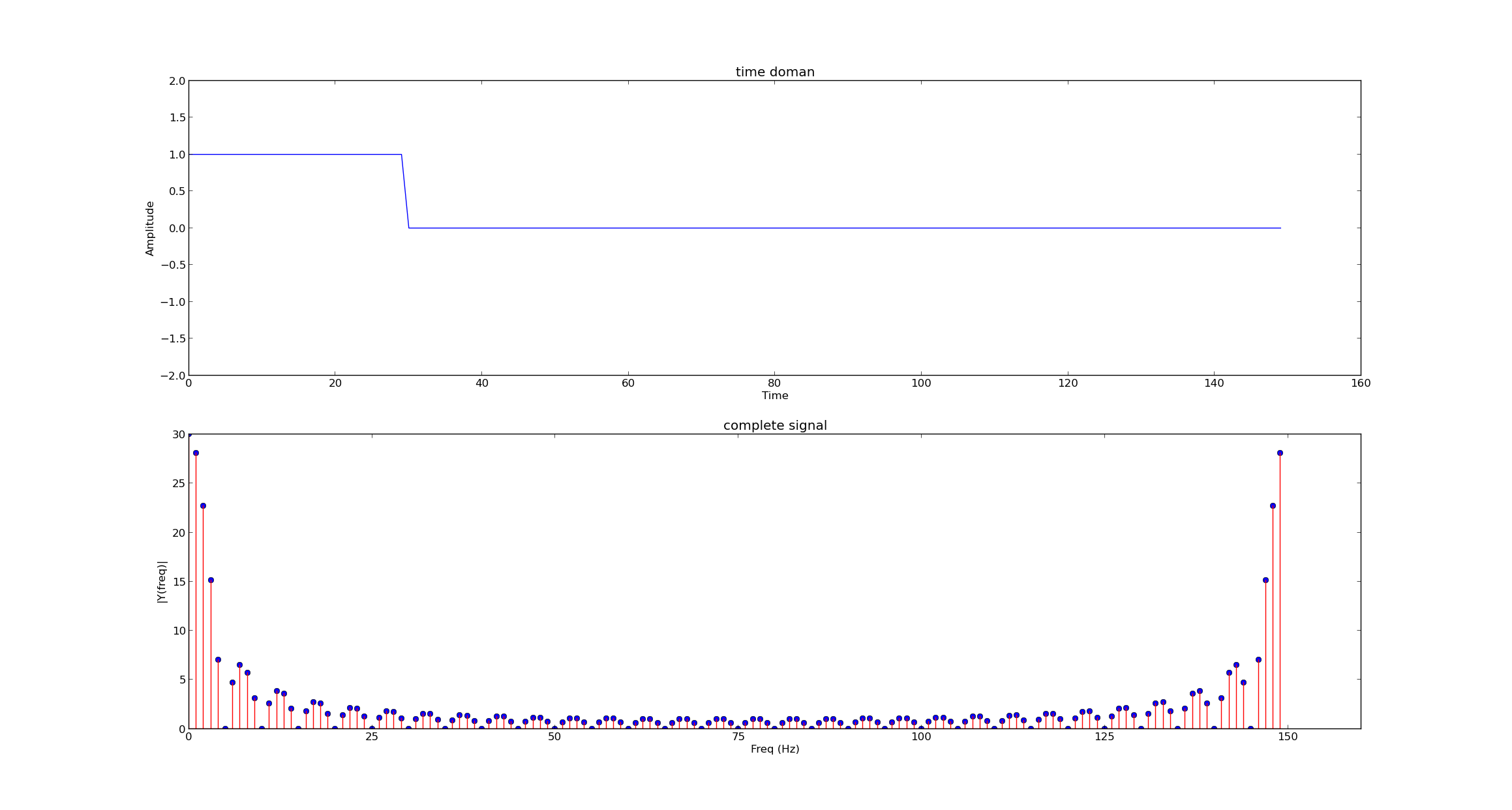
At we increase the period of the signal we can see that resolution in the freuency domain increases.
As $N \rightarrow \infty$ ,the samples in the freuency domain will be placed closer and closer . If samples in frequency domain are spaced infinitely closely,it can be considered a continuous signal. This gives us Discrete Time Fourier Transform representation of the signal.
def FourierRect(N):
        """ the function generates rectangular aperiodic pulse and computer the DFT coefficients

        Parameters
        ----------
        N : period of aperiodic signal

        """
        x = np.zeros((1,N))
        x[:,0:30]=1;
        x=x.flatten();


        #compute the DFT coefficients
        r1=FourierSeries(x)
        #magnitude of DFT coefficients
        a1=cabs(r1)

        #plot the time domain signal
        subplot(2,1,1)
        plt.plot(range(0,len(x)),x)
        xlabel('Time')
        ylabel('Amplitude')
        title('time doman')
        plt.ylim(-2,2);

        #plot the DFT coefficients
        L=len(a1);
        fr=np.arange(0,L);
        subplot(2,1,2)
        plt.stem(fr,a1,'r') # plotting the spectrum
        xlabel('Freq (Hz)')
        ylabel('|Y(freq)|')
        title('complete signal')
        ticks=np.arange(0,L+1,25);
        plt.xticks(ticks,ticks);
        show()

    if mode==4:
       FourierRect(150);

    if mode==5:
       FourierRect(150*3);
It samples in frequency domain are spaced infinitely closely,it can be considered a continuous signal. This representation of is called as Fourier Transform.
\[X(k) = \sum x[n] exp(-j\omega k n)\]distance between adjacent samples is $\omega$ .As $ w \rightarrow 0 $ samples are placed infinitely closely with each other .
\[X(w) = \sum x[n] exp(-j\omega n)\]Fourier transform is continuous in nature and cannot be used for numeral computation .
Discrete Fourier transform is sampled version of Discrete Time Fourier transform of a signal and in in a form that is suitable for numerical computation on a signal processing unit.
A fast Fourier transform (FFT) is an algorithm to compute the discrete Fourier transform (DFT) and its inverse.It is a efficient way to compute the DFT of a signal.
we will use the python FFT routine can compare the performance with naive implementation
Using the inbuilt FFT routine :Elapsed time was 6.8903e-05 seconds
Using the naive code :Elapsed time was 0.0653119 seconds
we can see improvement of order of 1000
The naive algorithm has complexity of $o(N^2)$ and FFT algorithm as complexity of $O(N log N)$
    if mode==6:
        Fs=150;
        F=range(1,10);
        F=np.array(F);
        w=numpy.ones(F.shape);


        Ts=1.0/Fs;
        xs=numpy.arange(0,1,Ts)

        signal=numpy.zeros(np.shape(xs));
        for i in range(len(F)):
            omega=2*np.pi*F[i];
            signal = signal+ w[i]*numpy.cos(omega*xs);


        start_time = time.time()
        FourierSeries(signal)
        end_time = time.time()
        print("Elapsed time naive algo  %g seconds" % (end_time - start_time))

        start_time = time.time()
        fft(signal)
        end_time = time.time()
        print("Elapsed time of fft algo  %g seconds" % (end_time - start_time))
Circular Convolution and DFT
Circular Shift of a sequence
Let $x[n]$ denote the finite length time domain sequence
Once we take DFT ,in time domain we are constructing the periodic extension of the signal Thus a time shit of signal is actually implies circular shit of the signal.
\(x[n] \Leftrightarrow X[k]\) \(x[(n-n\_{o})\_{N}] \Leftrightarrow e^{-j k \omega n\_{o}} X[k]\)
One of the most basic application in signal processing is linear convolution.
It can be used to represents the output of discrete time LTI system,correlation and cross correlation, filtering and host of other signal processing operations.
Linear Convolution in discrete time system is represented as
\[y[n]=\sum\_{i} x[i] h[n-i]\]The signals $x[n]$ and $h[n]$ are finite duration discrete time signals .
Linear convolution of 2 sequences of length M,L results in sequence of length M+L-1
An associated discrete time Fourier transform property
\[Y\left(\Omega\right) = X\left(\Omega\right)H\left(\Omega\right)\]Let us consider 2 sequences,take their DFT,multiply them and then take the inverse
Circular convolution in time domain leads to multiplication of DFT coefficients in the frequency domain
lets take the seuences [1,1,1,1,1] and [1,2,3,4]
The result of linear convolution is `[ 1  3  6 10 10  9  7  4 ]`
The result of inverse of product of DFT coefficients is `[ 10.  10.  10.  10.  10.]`
we take N point DFT of signals,N=max(M,L)
...|1 1 1 1 1|1 1 1 1 1|1 1 1 1 1|....
...|1 2 3 4 0|1 2 3 4 0|1 2 3 4 0|....
Result
...|10|10|10| ...
Taking the DFT leads to periodicity in time domain,now we perform convolution as usual. the $h[n-n_{o}]$ will be circularly shifted
...|1 1 1 1 1|1 1 1 1 1|1 1 1 1 1|....
...|0 1 2 3 4|0 1 2 3 4|0 1 2 3 4|....

Result
...|10|10|10| ...
...|1 1 1 1 1|1 1 1 1 1|1 1 1 1 1|....
...|4 0 1 2 3 |4 0 1 2 3|4 0 1 2 3|....

Result
...|10|10|10| ...
After N shifts we are repeating the sequence Thus we perform the convolution of N shifts equivalent to the period of sequence in time domain
Circular convolution
[ 10.  10.  10.  10.  10.]
Circular shift is consequence of periodicity introduced by the DFT and results in circular convolution operation
We can consider this due to the time aliasing being introduced due to sampling in the frequency domain. The sampling theorem states that to avoid aliasing in frequency domain the sampling rate must be greater than twice the maximum frequency of signal being sampled.
We had mentioned earlier that DFT is the sampled version of DTFT .The question arises that how do we increase the sampling rate to avoid time domain aliasing.
We saw that zero padding the sequence leads to samples of Fourier series are placed more closely together.Equivalent to saying increases the sampling rate of DTFT in frequency domain,
This gives us a intuition that if we zero pad the sequence,it will lead to increased sampling rate of the DTFT of the signal.
For the result of circular convolution to be equal to the linear convolution,we simply zero pad the sequences to length of M+L-1.
...|1 1 1 1 1 0 0 0 0 |1 1 1 1 1 0 0 0 0 |
...|1 2 3 4 0 0 0 0 0 |1 2 3 4 0 0 0 0 0 |

result : 10

...|1 1 1 1 1 1 0 0 0 |1 1 1 1 1 0 0 0 0 |
...|0 1 2 3 4 0 0 0 0 |0 1 2 3 4 0 0 0 0 |

result : 10

...|1 1 1 1 1 1 0 0 0 |1 1 1 1 1 0 0 0 0 |
...|0 0 1 2 3 4 0 0 0 |0 0 1 2  3 4 0 0 0 |

result : 9
thus we can see that due to zero padding,the circular shifted components are zeros and the result obtained is equivalent to linear convolution result.
The code for the above example is given below
    if mode == 7:
        x=np.array([1,1,1,1,1]);
        h=np.array([1,2,3,4,0]);
        r=np.convolve(x,h)
        print 'Linear convolution'
        print r

		#take 5 point DFT of the sequence
        f1=fft(x,5);
        f2=fft(h,5);
        s=ifft(f1*f2);
        print 'Circular convolution'
        print abs(s)

		#take 9 point DFT of sequence
        f1=fft(x,9);
        f2=fft(h,9);
        s=ifft(f1*f2);
        print 'zero padded Circular convolution'
        print r
Code
The code for all the examples can be found at github repository https://github.com/pi19404/pyVision/tree/master/pySignalProc/tutorial/fourierSeries.py
You can change the mode variable in the file from 1-7 to generate all the plots shown in the article
The file fourierSeries.py can also be downloaded from below link