Multilayer Perceptron in Python
03 Oct 2014Introduction
In this article we will look at supervised learning algorithm called Multi-Layer Perceptron (MLP) and implementation of single hidden layer MLP
###Perceptron
A perceptron is a unit that computes a single output from multiple real-valued inputs by forming a linear combination according to its input weights and then possibly putting the output through some nonlinear function called the activation function
Below is a figure illustrating the operation of perceptron
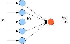
The output of perceptron can be expressed as
$f(x) = G( W^T x+b)$
$x$ is the input vector $(W,b)$ are the parameters of perceptron $f$ is the non linear function
Multi Layer Perceptron
The MLP network consists of input,output and hidden layers.Each hidden layer consists of numerous perceptron’s which are called hidden units
Below is figure illustrating a feed forward neural network architecture for Multi Layer perceptron
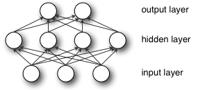
A single-hidden layer MLP contains a array of perceptrons . The output of hidden layer of MLP can be expressed as a function
$f(x) = G( W^T x+b)$
$f: R^D \rightarrow R^L$, where D is the size of input vector $x$ $L$ is the size of the output vector $G$ is activation function.
In case the activation function G is a sigmoid function then a single-layer MLP consisting of just the output layer is equivalent to a logistic classifier
$\begin{align} f_{i}(x)=\frac{e^{W_{i}x+b_{i}}}{\sum_{j} e^{W_{j}x+b_{j}}} \end{align}$
Each unit of input layer corresponds to element of input vector. Each output unit of logistic classifier generate a prediction probability that input vector belong to a specified class.
##Feed Forward Neural Network Let us first consider the most classical case of a single hidden layer neural network
The number of inputs to hidden layer is $(d)$ and number of outputs of hidden layer are $(m)$ The hidden layer performs mapping of vector of dimensionality $d$ to vector of dimensionality $m$.
Each unit of hidden layer of a MLP can be parameterized by a weight matirx and bias vector $(W,b)$ and a activation function $(\mathcal{G})$.The output of a hidden layer is activation function applied to linear combination of input and weight vector.
Dimensionality of weight matrix and bias vector are determined by desired number of output units. If the number of inputs to hidden layer/dimensionality of input is $\mathcal{M}$ and number of outputs is $\mathcal{N}$ then dimensionality of weight vector in $\mathcal{NxM}$ and that of bias vector is $\mathcal{N}x1$.
We can consider that hidden layer consists of $\mathcal{N}$ hidden units ,each of which accepts a $\mathcal{M}$ dimensional vector and produces a single output.
The output is the affine transformation of the input layer followed by the appplication of function $f(x)$ ,which is typically a non linear function like sigmoid of inverse tan hyperbolic function.
The vector valued function $h(x)$ is the output of the hidden layer.
\[h(x) = f(W^T x + c )\]The output layer of MLP is typically Logistic regresson classifier,if probabilistic outputs are desired for classification purposes in which case the activation function is the softmax regression function.
###Single Hidden Layer Multi Layer Perceptron’s Let ,
- $h_{i-1}$ denote the input vector to the i-th layer
- $h_{i}$ denote the output vector of the i-th layer.
- $h_{0}$=x is vector that represents input layer
- $h_{n}=y$ is output layer which produces the desired prediction output.
- $f(x)$ denote the activation function
Thus we denote the output of each hidden layer as
$h_{k}(x) = f(b_{k} + w_{k}^T h_{i-1}(x)) = f(a_{k}) $
Considering sigmoid activation function,gradient of fundtion wrt arguments can be written as
$\begin{align} \frac{\partial \mathbf{h}_{k}(x) }{\partial \mathbf{a}_{k}}= f(a_{k})(1- f(a_{k})) \end{align}$
The computation associated with each hidden unit $(i)$ of the layer can be denoted as
\[h\_{k,i}(x) = f(b\_{k,i} + W\_{k,i}^T h\_{i-1}(x)) = f(a\_{k}(x))\]The output layer is a Logistic regression classifier.The output is a probabilistic output denoting the confident that input belongs to the predicted class.The cost function defined for the same is defined as negative log likelyhood over the training data
\[L = -log (p\_{y})\]The idea is to maximize $p_{y}= P( Y =y_{i} | x )$ as estimator of conditional probability of the class $y$ given that input is $x$.This is the cost function for training algorithm.
###Back-Propagation Algorithm
The Back-Propagation Algorithm is recursive gradient algorithm used to optimize the parameters MLP wrt to defined loss function.Thus our aim is that each layer of MLP the hidden units are computed so that cost function is maximized.
Like in logistic regression we compute the gradients of weights wrt to the cost function . The gradient of the cost function wrt all the weights in various hidden layers are computed.Standard gradient based optimization is performed to obtain the parameters that will minimize the likelihood function.
The output layer determines the cost function.Since we are using Logistic regression as output layer.The cost function is the softmax function.Let L denote the cost function.
There is nothing different we do in backpropagation algorithm that any other optimization techniue.The aim is to determine how the weights and biases change in the network
$ \begin{align} \frac{\partial L}{\partial W_{k,i,j} } \text{ and } \frac{\partial L}{\partial b_{k,i,j} } \end{align}$.
output layer
$\begin{align} L = -log ( f(a_{k,i}) ) \end{align}$
$\begin{align} \frac{\partial L }{\partial \mathbf{a}_{k,i}} = \frac{\partial L }{\partial \mathbf{h}_{k,i}} \frac{\partial \mathbf{h}_{k,i} }{\partial \mathbf{a}_{k,i}} = -\frac{1}{h_{k,i}} * h_{k,i}*(1-h_{k,i}) = (h_{k,i}-1)\end{align} $
$ \begin{align} \frac{\partial L }{\partial \mathbf{a}_{k,i}} =\mathbf{h}_{k,j} - 1_{y=y_{i}} \end{align}$
The above expression can be considered as the error in output.When $y=y_{i}$ the error is $(1-p_{i})$ and then $y \ne y_{i}$ the error in prediction is $p_{i}$.
hidden layer
$\begin{align}\frac{\partial L }{\partial \mathbf{a}_{k-1,j}} = \frac{\partial L }{\partial \mathbf{h}_{k-1,j}} \frac{\partial \mathbf{h}_{k-1,j} }{\partial \mathbf{a}_{k-1,j}} \end{align}$
Thus the idea is to start computing gradients from the bottom most layer.To compute the gradients of the cost function wrt parameters at the i-th layer we need to know the gradients of cost function wrt parameters at $(i+1)$th layer.
We start with gradient computation at the logistic classifier level.The propagate backwards,updating the parameters at each layer
Let us consider the case of other other hidden layers
$\begin{align} \frac{\partial L }{\partial \mathbf{h}_{k-1,j}} = \sum_{i} \frac{\partial L }{\partial \mathbf{a}_{k,i}}\frac{\partial \mathbf{a}_{k,i} }{\partial \mathbf{h}_{k-1,j}} = \sum_{i} \frac{\partial L }{\partial \mathbf{a}_{k,i}} W_{k,i,j} \end{align} $
The implementation of the above equation
    def linear_gradient(self,weights,error):
            """ The function compues gradient of likelihood function wrt output of hidden layer
            :math:`\\begin{align} \\frac{\partial L }{\partial \mathbf{h}\_{k-1,j}} \\end{align}`

            Parameters
            ------------
            weights : ndarray,shape=(n_out,n_hidden)
                      weights of next hidden layer, :math:`\\begin{align} \mathbf{W}\_{k,i,j}  \\end{align}`

            error   : ndarray,shape=(n_out,)
                      backpropagated error from next layer :math:`\\begin{align} \\frac{\partial L }{\partial \mathbf{a}\_{k,i}} \\end{align}`

            Returns
            -----------
            out : ndarray,shape=(n_hidden,)
                  compute the backpropagated error, :math:`\\begin{align} \\frac{\partial L }{\partial \mathbf{h}\_{k-1,j}} \\end{align}`
            """

            return numpy.dot(error,weights);
The gradients computation of parameters of hidden layers is as follows
$\begin{align}\frac{\partial L }{\partial \mathbf{W}_{k-1,i,j}} = \frac{\partial L }{\partial \mathbf{a}_{k-1,j}} \frac{\partial \mathbf{a}_{k-1,j} }{\partial \mathbf{W}_{k-1,i,j}}=\frac{\partial L }{\partial \mathbf{a}_{k-1,j}} \mathbf{h}_{k-2,j} \end{align}$
$\begin{align}\frac{\partial L }{\partial \mathbf{b}_{k-1,i}} = \frac{\partial L }{\partial \mathbf{a}_{k-1,i}} \frac{\partial \mathbf{a}_{k-1,i} }{\partial \mathbf{b}_{k-1,i}}=\frac{\partial L }{\partial \mathbf{a}_{k-1,i}} \end{align}$
This is implemented as below ,where the input
- $x$ represents $\begin{align} \frac{\partial \mathbf{h}_{k,j} }{\partial \mathbf{a}_{k,j}} \end{align}$ -output gradient
- $y$ represents $\begin{align} h_{k-2,j} \end{align}$ -activation
- $w$ represents $\begin{align} \frac{\partial L }{\partial \mathbf{a}_{k-1,i}}\end{align}$ -error
    def compute_error(self,x,w,y):
        """
        function computes the gradient of the likelyhood function wrt to parameters  of the hidden layer for single input


        Parameters
        -------------
        x : ndarray,shape=(n_hidden,)

        w : ndarray,shape=(n_hidden,)
            `w` represents :math:`\\begin{align} \\frac{\partial L }{\partial \mathbf{h}\_{k,i}}\end{align}` the gradient of the likelyhood fuction wrt output of hidden layer

        y : ndarray,shape=(n_in,)
            `y` represents :math:`\mathbf{h}\_{k-2,j}` the input hidden layer

        Returns
        ------------
        res : ndarray,shape=(n_in+1,n_hidden)
              :math:`\\begin{align} \\frac{\partial L }{\partial \mathbf{W}\_{k-1,i,j}}  \\text{ and } \\frac{\partial L }{\partial \mathbf{W}\_{k-1,i}} \end{align}`
        """


        x=x*w;
        #gradient of likelyhood function wrt input activation
        res1=x.reshape(x.shape[0],1);
        #gradient of likelyhood function wrt weight matrix
        res=np.dot(res1,y.reshape(y.shape[0],1).T);
        self.eta=0.0001
        #code for L1 and L2 regularization
        if self.Regularization==2:
           res=res+self.eta*self.W;
        if self.Regularization==1:
           res=res+self.eta*np.sign(self.W);

        #stacking the parameters and preparing for returning
        res=np.hstack((res,res1));
        return res.T;


    def cost_gradients(self,weights,activation,error):
        """ function to compute the gradient of log
        likelyhood function wrt the parameters of the hidden layer
        averaged over all the input samples.

        Parameters
        -------------
        weights : numpy,shape(n_out,n_hidden),
                  weight matrix of the next layer,W\_{k,i,j}


        activation: numpy,shape=(N,n_in)
                    input to the hidden layer \mathbf{h}\_{k-2,j}

        error : numpy,shape=(n_out,)
                 \frac{\partial L }{\partial \mathbf{a}\_{k,i}}

        Returns

        -------------
        gW : ndarray,shape=(n_hidden,n_in+1)
             coefficient parameter matrix of next hidden layer,
             :math:`\\begin{align} \\frac{\partial L }{\partial \mathbf{W}\_{k-1,i,j}}  \\text{ and } \\frac{\partial L }{\partial \mathbf{W}\_{k-1,i}} \end{align}`
        """
        we=self.linear_gradient(weights,error)
        ag=self.activation_gradient()
        e=[ self.compute_error(a,we,b) for a,b in izip(ag,activation)]
        gW=np.mean(e,axis=0).T
        return gW;
Once we have the gradients and have computed the new parameters,the function update is called to updated the new parameters in the model.
This function is called by the Optimizer module that performs SGD based optimizations,all the optimization parameters like learning rate are handled by the optimizer methods.
    def update_parameters(self,params):
        """ function to updated the learn parameters to the model

        Parameters
        ----------
        grads : ndarray,shape=(n_hidden,n_in+1)
                coefficient parameter matrix

        """

        self.params=params;
        param1=self.params.reshape(-1,self.nparam);
        self.W=param1[:,0:self.nparam-1];
        self.b=param1[:,self.nparam-1];
Implementation Details
The class HiddenLayer encapsulates all the methods for prediction,classification,training,gradient computation and error propagation that are required
The important attributes of the HiddenLayer class are
    Attributes
    -----------
    `out` : array-like ,shape=[n_out]
    The output of hidden layer

    `params`:array-like ,shape=[n_out,n_in+1]
     parameters of hidden layer

    `W,b`:array-like,shape=[n_out,n_int],shape=[n_out,1]
     parameters in the form of weight matrix and bias vector characterizing
     the hidden layer

     `activation`:function
     the non linear activation function

    .. note :
    in the below functions to n_hidden denotes the number of output units of present hidden layer
    n_out denotes the number of output units of next hidden layer
    and n_in denotes the size of input vector to present hidden layer

    def compute(self,input):
        """function computes the output of the hidden layer for input matrix

        Parameters
        ----------
        input   :   ndarray,shape=(N,n_in)
                    :math:`h\_{i-1}(x)` is the `input`

        Returns
        -----------
        output  : ndarray ,shape=(N,n_out)
                    :math:`f(b_k + w_k^T h\_{i-1}(x))` ,affine transformation over input
        """
        #performs affine transformation over input vector
        linout=numpy.dot(self.W,input.T)+np.reshape(self.b,(self.b.shape[0],1));
        #applies non linear activation function over computed linear transformation
        self.output=self.activation(linout).T;
        return self.output;
A class MLP encapsulates all the methods for prediction,classification,training,forward and back propagation,saving and loading models etc. Below 3 important functions are displayed.The learn function is called at every optimizer loop. This calls the forward and backward iteration methods and updated the parameters of each hidden layer
the forward iteration simply computes the output of network and while propagate_backward fuctions is responsible for passing suitable inputs and weights to each hidden layer so that it can execute the backward algorithm loop
   def propagate_backward(self,error,weights,input):
        """ the function that executes the backward propagation loop on hidden layers

        Parameters
        ----------------
        error : numpy array,shape=(n_out,)
                average prediction error over all the input samples in output layer
                :math:`\\begin{align}\frac{\partial L  }{\partial \mathbf{a}\_{k,i}} \\end{align}`


        weight : numpy array,shape=(n_out,n_hidden)
                 parameter weight matrix of the output layer


        input : ndarray,shape=(n_samples,n_in)
                input training data
        Returns
        ----------------
        None

        """


        #input matrix for the hidden layer
        input1=input;
        for i in range(self.n_hidden_layers):
            prev_error=np.inf;
            best_grad=[];
            for k in range(1):
                """ computing the derivative of the parameters of the hidden layers"""
                hidden_layer=self.hiddenLayer[self.n_hidden_layers-i-1];
                hidden_layer.compute(input1);

                # computing the gradient of likelyhood function wrt the parameters of the hidden layer
                grad=hidden_layer.cost_gradients(weights,input1,error);
                #update the parameter of hidden layer
                res=self.update(hidden_layer.params,grad.flatten(),0.13);

                """ update the parameters """
                hidden_layer.update_parameters(res);
            #set the weights ,inputs and error required for the back propagation algorithm
            #for the next layer
            weights=hidden_layer.W;
            error=grad[:,hidden_layer.n_in];
            self.hiddenLayer[self.n_hidden_layers-i-1]=hidden_layer;
            input1=hidden_layer.output;

   def propagate_forward(self,input):
       """the function that performs forward iteration to compute the output

       Parameters
       -----------
       input : ndarray,shape=(n_samples,n_in)
               input training data

       """
       self.predict(input)


   def learn(self,update):
        """ the main function that performs learning,computing gradients and updating parameters
            this is called by the optimizer module for each iteration

        Parameters
        ----------
        update - python function
                 this represents the update function that performs the gradient descent iteration
        """
        #set the training data
        x,y=self.args;
        #set the update function
        self.update=update;
        #execute the forward iteration loop
        self.propagate_forward(x)
        #set the input for output layer
        args1=(self.hidden_output,y);
        #set the input for the output logistic regression layer
        self.logRegressionLayer.set_training_data(args1);
        #gradient computation and parameter updation of output layer
        [params,grad]=self.logRegressionLayer.learn(update);
        self.logRegressionLayer.update_params(params);

        #initialize the gradiients and weights for backward error propagation
        error=grad;
        weights=self.logRegressionLayer.W;

        #perform the backward iteration over the hidden layers
        if self.n_hidden_layers >0:
             weights=self.logRegressionLayer.W;
             self.propagate_backward(error,weights,x)

        return [None,None];
Selecting the parameters of the model
As mentioned earlier that MLP consits of input,hidden and output layers.There is not fixed rule to determine the number of hidden units.The parameters are application specific and best parameters are often arrived at by emperical testing process.Less number of hidden units leads to increased generalization and training error while having a large number of training units leads to issues of with training of large number of parameters and significantly large training time.
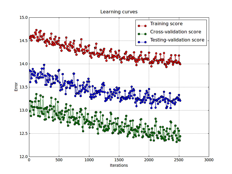
Issues with MLP
One of the issues observed in MLP training is the slow nature of learning.The below figure illustrates the nature of learning process when a small learning parameter or improper regularization constant is chosen.Various adaptive methods can be implemented which can improve the performance ,but slow convergence and large learning times is an issue with Neural networks based learning algorithms.
Code
The important files related to MLP are
- MLP.py
- LogisticRegression.py
- Optimizer.py
The latest version of the code can be found in github repository www.github.com/pi19404/pyVision
The files used in the current article can be downloaded from below link
The dataset and model file can be found under the models and data repository
- MLP.pyvision - model file
- mnist.pkl.gz - data file
make suitable changes to the path in MLP.py file before running the code.