Conjugate Quadrature Filter Bank - Deriving Daubechies Filter Coefficients
21 Dec 2014Introduction
In this article we will look at the concept of conjugate quadrature filter bank and process computationally derive the Daubechies wavelet filter coefficient for any filter length
Conjugate Quadrature Filters (CQFs)
Following up on the Perfect Reconstruction Filter Banks.In this article we will look at look at realization of perfect reconstruction filter bank using Conjugate Quadrature Filters.
Let $x[n]$ represent a real sequence and $X(z)$ represent the Z transform.
Conjugate Filter
$X(z) = \sum x[n] z^{-k}$ $Y(z) = X^{*}(Z)=\sum x[n] z^{k} = X(z^{-1})$ $y[n] = x[N-n]$
Quadrature Filters
If $Y(z) = H_{0}(-z)$ $y[n] = \sum_{k} (-1)^{k} h_{o}[k] = (-1)^{n}h_{o}[n]$
The filter responses are symmetric about $\Omega = \pi / 2$
| $ | Y(e^{j\Omega}) | = | Y(e^{j(\pi - \Omega)}) | $ |
Conjugate Quadrature Filters
The relation between the analysis HPF (high pass filter) and analysis LPF (low pass filter) of the filter bank forms conjugate quadrature relationship
$H_{1}(z) = z^{-d}H_{0}(-z^{-1})$
$G_{0}(z) = H_{1}(-z)$
$G_{1}(z) = -H_{0}(-z)$
$h_{1}(n) = \sum_{k=0}^{N} h_{0}(N-k-d)(-1)^{k} $
$ z^{-d}$ is used to introduce causality
$H_{1}(e^{j\omega}) = e^{-j\omega d}H_{0}(-e^{-j\omega}) $
Magnitude response is given by $|H_{1}(e^{j\omega})| = |H_{0}(-e^{-j\omega})| $
if $H_{0}(z)$ is a low pass filter with real impulse response then $H_{0}(e^{-j\omega}) =H_{0}^{*}(e^{-j\omega})$
| $ | H_{1}(e^{j\omega}) | = | H_{0} | (e^{-j(\omega+\pi)}) | $ |
Condition For Perfect Reconstruction
$T_{1}(z) =[H_{0}(z) H_{1}(-z) - H_{1}(z) H_{0}(-z)] =C_{0} z^{-D} $
$T_{1}(z) = H_{0}(z) {-z}^{-d}H_{0}(z^{-1}) - z^{-d}H_{0}(-z^{-1})H_{0}(-z)=c_{0}z^{-d}$
${-1}^{d} H_{0}(z) H_{0}(z^{-1}) - H_{0}(-z^{-1})H_{0}(-z) = C_{0}$
if D is odd
$ H_{0}(z) H_{0}(z^{-1}) + H_{0}(-z^{-1})H_{0}(-z) = C_{0}=2$
$ H_{0}(e^{j\omega}) H_{0}(e^{-j\omega}) + H_{0}(-e^{-j\omega})H_{0}(-j\omega) = C_{0}=2$
For real impulse response
| $ | H_{0}(e^{j\omega}) | ^2 + | H_{0}(e^{-j(\omega+\pi)}) | ^2 = C_{0}=2$ |
$K_{0}(z) = H_{0}(z) H_{0}(z^{-1}) $
| $K_{0}(e^{j\omega}) = H_{0}(e^{j\omega}) H_{0}(e^{-j\omega}) = | H_{0}(z) | ^2$ |
$K_{0}(-z) = H_{0}(-z) H_{0}(-z^{-1}) $
| $K_{0}(-e^{j\omega}) = H_{0}(-e^{j\omega}) H_{0}(-e^{-j\omega}) = | H_{0}(-z) | ^2$ |
With odd D
$K_{0}(z)+ K_{0}(-z)= C_{0}=2$
with even D
$K_{0}(z)- K_{0}(-z) = C_{0}=2$
Normalization Constraint
$ x[n] \Rightarrow X(z) $
$ x[-n] \Rightarrow X(z^{-1}) $
$K_{0}(z) = H_{0}(z) H_{0}(z^{-1}) $ are convolution of signal $h_{0}[n]$ and $h_{0}[-n]$ which is correlation function $R_{k}[n]$ which is symmetrical
$K_{0}(-z) = H_{0}(-z) H_{0}(-z^{-1}) $ are convolution of signal $h_{0}[n]e^{j\pi n}$ and $h_{0}[-n]e^{-j\pi n}$ which is correlation function $R_{k}[n]e^{j\pi n}$ which is symmetrical
These give rise to
Square Normalization Constraint
$\sum_{n} h_{0}^2[n] =1$
Scaling Function Constraint We impose a constraint that scaling function has unit area
$\phi(t) = \sum_{k} h_{0}[k] \phi[2t-k]$ $\int \phi(t) dt = \int \sum_{k} h_{0}[k] \phi[2t-k]$ dt $
Normalization Constraint
$\sum_{n} h_{0}[n] = \sqrt{2}$
Conditions for Perfect Reconstruction For perfect reconstruction filter banks we need to select $H_{0}(z)$ which will satisfy the condition
With odd D
$K_{0}(z)+ K_{0}(-z)= C_{0}$
with even D $K_{0}(z)- K_{0}(-z) = C_{0}$
From the above equation the summation $K_{0}(z)+ K_{0}(-z)$ represents the nonzero sample value at even location and zero sample value at the odd location.
Let $k_{0}[n]$ correspond to the sequence $K_{0}(z)$.The requirement is that we only want non zero value at zero location and zero value at all other locations
This gives rise to
Even shift orthogonality
$\sum_{k=0}^{N-1} h_{0}[k]h_{0}[k-2l] = 0 ,\forall l \ne 0 $
Let $k_{0}[n]$ correspond to the sequence $K_{0}(z)$.The requirement is that we only want non zero value at zero location and zero value at all other locations
This gives rise to
Even shift orthogonality
$\sum_{k=0}^{N-1} h_{0}[k]h_{0}[k-2l] = 0 ,\forall l \ne 0 $
The two additional constrains on the filter moments are due to vanishing moment constrain seen in the article Approximation of Piecewise Polynomial Using Wavelets
Zero order vanishing moment constraint
$\sum\_{k} (-1)^{k} h(k) =0$
pth order vanishing moment constraint
$\sum\_{k} (-1)^{k} k^{p}h(k) =0$
Thus the constraints imposed on filter coefficients like square normalization,normalization,vanishing moments and even shift orthogonality are consequence or requirement of perfect reconstruction filter bank
Daubechies Family of Wavelets
Daubechies is a class of wavelets belonging to class of Conjugate Quadrature Filters .
In Daubechies family of wavelets the idea is to have more $(1 − z^{−1}) $ terms on the high pass branch. Daubechies wavelet filters bank are realization of type of filter bank called Conjugate Quadrature Filter bank.
As a example let us consider a filter of length 4 (Daubechies 2 Wavelets) As mentioned we are seeking a filter that has 2 $(1-z^{-1})$ terms on it high pass branch
The filter is of the form
$H_{1}(z) = z^{-d}H_{0}(-z^{-1})$
That means the low pass filter will have 2 $(1+z^{-1})$ terms on it high pass branch
$H_{0}(z)=h_{0}+ h_{1}z^{-1} + h_{2}z^{-2}+h_{3}z^{-3}$
$H_{0}(z)=(1+z^{-1})^2(1+B_{0}z^{-1})$
$H_{0}(\omega) =( {1+e^{-j\omega}})^2 L(\omega)$
$H_{0}(\pi) =0 $
This constraint comes from above condition
Vanishing moment Constraint
$H_{0}(\pi) =0 $ $h_{0} - h_{1} + h_{2} - h_{3} =0$
$H_{0}(z)=(1+2z^{-1}+z^{-2})(1+B_{0}z^{-1})$
$H_{0}(z)=1+(2+B_{0})z^{-1}+(1+2B_{0})z^{-2}+B_{0}z^{-3}$
$h_{0}[n]=C_{0}[ 1 , (2+B_{0}) ,(1+2B_{0}) , B_{0} ]$
The even values of autocorrelation function should be 0
$R(2) = (1+2B_{0}) +(2+B_{0})B_{0}=0$
$R(2) = $B_{0}^{2}+ 4 B_{0} + 1=0$
solving we get
$B_{0} = -2 + \sqrt{3} =-0.268$
we also get
$h_{0}[n] = C_{n}[1,1.732,0.464,-0.268]$
$R(0) = 0.4829$
Thus we have $C_{0}=\frac{1}{0.4829}$
$h_{0}[n] = [0.4829,0.8364,0.2241,-0.129]$
The filter coefficient is said to belong to family of Daubechies wavelts .And since the high has filter has 2 zeros it is called as daub-2 wavelet.
For example in the above case we have
$h_{0}^{2}+ h_{1}^{2} + h_{2}^{2}+h_{3}^{2}=1$
$h_{0}+ h_{1} + h_{2}+h_{3}=\sqrt{2}$
$h_{0}h_{2}+ h_{1}h_{3}=0$
$h_{0} - h_{1} + h_{2} - h_{3} =0$
$0*h_{0} - h_{1} + 2 h_{2} - 3 h_{3} =0$
The next member of Daubechies family is a length 6 filter of degree 5.And $H_{0}(z)$ can be written as
$H_{0}(z)=(1+z^{-1})^3(1+B_{0}z^{-1})(1+B_{1}z^{-1})$
we can solve for the coefficient using the same method as above
This type of filter banks are called Conjugate Quadrature filter bank. The reason for this nomenclature is that the low pass and the high pass filter frequency responses are $\pi$ apart from each other and are governed by the constraint
$K_{0}(z)+ K_{0}(-z)= C_{0}$
Typically the Daubechies can be defined for any filter size.
However we need a computationally way to derive these equations.The equations have a nonlinear constraint due to double shift orthogonality .The approach described above is not a scalable approach for higher filter sizes.
Computing the Wavelet Coefficients
We know that if a filter has $p$ zeros at $\pi$ it has 2 vanishing moments and total filter length if $2p$ and transfer function will have $2p-1$ zeros
The product filter $K_{0}(z)$ will have impulse response $4p-1$ coefficients and transfer function will have $4p-2$ zeros
for example
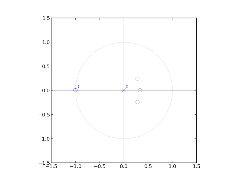
$h_{0}[n]=[-0.1294, 0.2241, 0.8365, 0.48296]$
$H_{0}(z)=-0.1294,+0.2241z^{-1}+0.8365z^{-2}0.48296z^{-3}$
$k_{0}[n]=[ 0.01674682, -0.0580127 , -0.16626588 , 0.25 , 0.91626588 , 0.8080127,0.23325318]$
The pole zero plot of $h_{0}[n],k_{0}[n]$ is shown below we can see that $h_{0}[n]$ has 3 zeros and $k_{0}[n]$ as 6 zeros
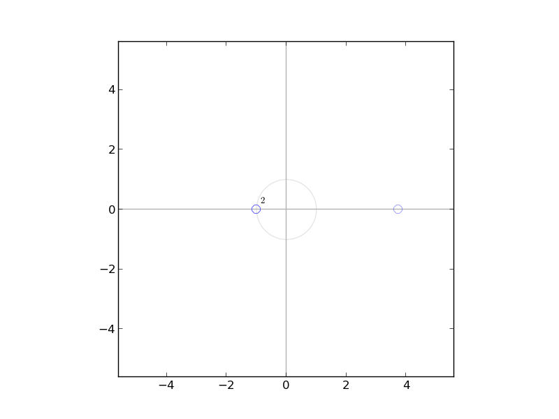

since $h(n)$ is real ,$h_{0}[Z]$ is a polynomial with real coefficients
Furthermore from complex conjugate theorem if a polynomial
$H(z) = a_{0} + a_{1}z + a_{2}z^2 + \cdots + a_{n} z^n$
has real coefficients, then any complex zeros occur in conjugate pairs. That is, if $a + bi$ is a zero then so is $a – bi$ and vice-versa.This is a direct implication that magnitude spectrum of polynomial with real coefficients is even symmetric.
This can be also seen in the below plot of arbitrary polynomial
$h[n]=[1,2,2,-1,5,4]$
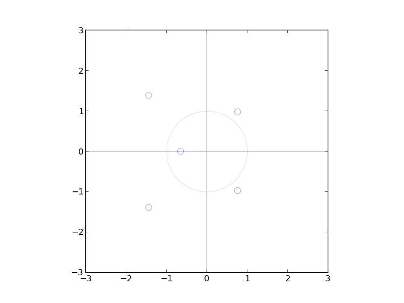
If $H(z)$ has p zeros then $K(z)=H(z)H^{}(z)$ will have 2p zeros
if $K(z)$ is real and even symmetric $K(z)=K^{}(z)=K(z^{})=K(z^{-1})$
if $z$ is a zero then $z^*=z^{-1}$ is also a zero
Thus $K_{0}(z)=H(z)*H^{* }(z)$ has zeros that come in quadrapulets of $z_{0},z^{*}_{0},\frac{1}{z_{0}},\frac{1}{z_{0}^{ * }}$ for complex zeros and duplets for real zero $z_{0},\frac{1}{z_{0}}$
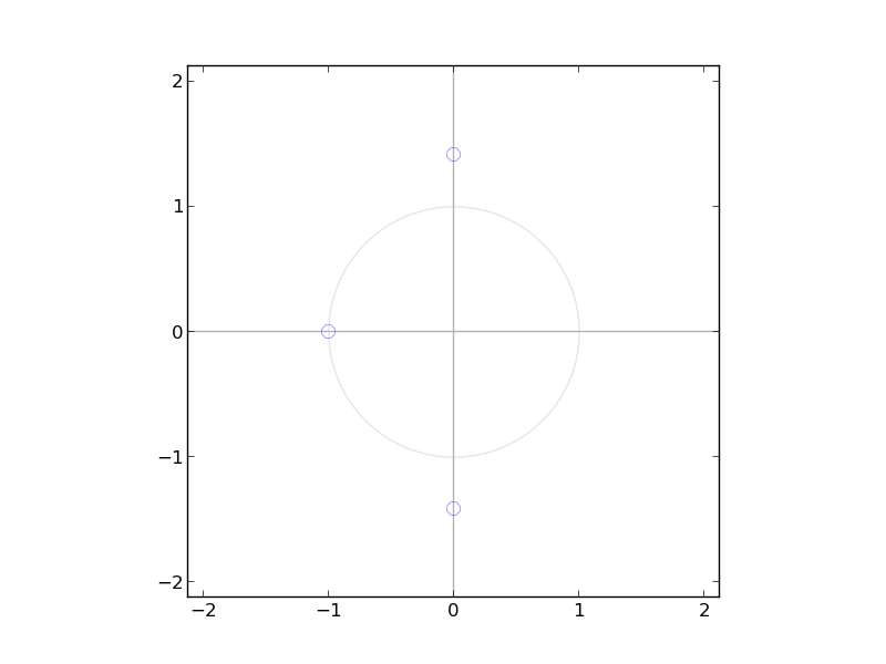
Again we take a arbitraty polynomial
$h[n]=[1,1,2,2]$
$k[n]=[ 2 , 4 ,7 ,10, 7 ,4 ,2]$
Let us assume that the frequency response of filter will take the form
$H_{0}(\omega) =( \frac{1+e^{-j\omega}}{2})^p L(\omega)$
The filter will have $p$ zeros at $\pi$ and let us assume that $L(\omega)$ is a polynomial which has a degree $p-1$ .
$L(\omega)$ is not unique . For any quadrapulet of complex zeros in $K(z)$.One can choose a pair of zeros to retain for construction of zeros in $L(z)$.Similarly for every duplet of real zeros there are 2 ways of choosing the $L(z)$
Thus there are total of $2^p$ different ways of choosing $L$.
| In the above example $ | L(w) | ^2$ contains zeros at $[j\sqrt{2},-j\sqrt{2},j\frac{1}{\sqrt2},-j\frac{1}{\sqrt2}]=[z1,z2,z3,z4]$ |
| $ | H_{0}(\omega) | ^2 =cos^2(\frac{\omega}{2})^p | L(\omega) | ^2$ |
In case of the above example the zeros are located at
$[j\sqrt{2},-j\sqrt{2},-1,-1,j\frac{1}{\sqrt2},-j\frac{1}{\sqrt2}]$
The zeros at $(-1)$ are not part of $L(\omega)$
| $ | L(w) | ^2$ contains zeros at $[j\sqrt{2},-j\sqrt{2},j\frac{1}{\sqrt2},-j\frac{1}{\sqrt2}]$ |
This can be written as
| $ | L(z) | ^2 = (z-j\sqrt{2})(z+j\sqrt{2})(z-j\frac{1}{\sqrt2})(z+j\frac{1}{\sqrt2})$ |
| $ | L(z) | ^2 = z^{4} + 2.5z^{2} +1$ |
It can also be seen that fourier transform of $K[z]$ can be written as polynomial of $cos(\omega)$
$K(\omega) = 2 e^{-j3\omega}[e^{-j3\omega}+4e^{-j2\omega} + 7 e^{-j\omega} + 10 + 2 e^{j3\omega}+4e^{j2\omega}+ 7 e^{j\omega} ]$
$K(\omega)= 2e^{-j3\omega}[4cos(2\omega ) + 7 cos(\omega ) + 10 + 2 cos(3\omega )]$
| $ | L(\omega) | ^2 = e^{j4\omega} + 2.5e^{j2\omega} + 1=e^{j2\omega}[2.5+2cos(2\omega)$ |
| $ | L(\omega) | ^2 =e^{j2\omega}[0.5 + 4 cos^2(\omega)]=e^{j2\omega}[16cos^2(\omega/2)-16cos(\omega/2)-3.5]$ |
This can be always expressed in the form of $sin^2(\omega/2)$
Again
| $ | H(e^{j\omega}) | ^2 + | H(e^{-j(\omega+\pi)}) | ^2=1$ |
if $y=cos^2(\omega/2)$ where $y \in [-1,1] $
Let us assume that $L(\omega)$ can always expressed as trigonometric polynomial interms of 1-y and $L(\omega+\pi)$ be expressed as polynomial of y.
The equation can be written as
$y^{p}F(1-y) + (1-y)^{p}F(y) = 1 ,\forall p $
This implies that any $H_{0}(\omega)$ satisfying the condition for perfect reconstruction corresponds to a polynomial $F(1-y)$ solving the above equation
Conversly every polynomial which satisfies the above equation will satisfy perfect reconstruction criteria and define the analysis filter of perfect reconstruction filter bank
A possible solution
An example of such a polynomial is
$F(y) = \frac{1}{2(1-y)^p} $
From binomial theorem we have
$\frac{1}{(1-x)^s} = \sum_{k=0}^\infty {s+k-1 \choose k} x^k \equiv \sum_{k=0}^\infty {s+k-1 \choose k} x^k = \sum_{k=0}^{p-1} {p+k-1 \choose k} x^{k} + O(x^p)$
This translates to
$1 + y^{k}O((1-y)^k) + (1-y)^{k} O(y^k) = 1$
or
$y^{k}O((1-y)^k) + (1-y)^{k} O(y^k)=0$
Let us take a finite number of terms of the series
$F_{p}(y) =0.5 \sum_{k=0}^p [{p+k \choose k} y^k]$
$F_{p}(1-y) = 0.5 \sum_{k=0}^p [{p+k \choose k} (1-y)^k]$
$S_{p} = 0.5 \sum_{k=0}^p {p+k \choose k} [{p+k \choose k} y^{p}(1-y)^k + y^{k}(1-y)^p ] $
Let $A_{n,j}$ represent the coefficient $jth$ term of the series
$A_{n,j} = 0.5{n+j\choose j} $
$A_{n,0} = 1 $
$(1-y)^{n+1} = (1-y)^n - y(1-y)^n $ $(y)^{n+1} = (y)^n - (1-y)(y)^n $
Now $S_{0} = 1$
$S_{p-1} = \sum_{k=0}^{p-1} A_{p-1,k}A_{p-1,j} [y^{p-1}(1-y)^k + y^{k}(1-y)^{p-1} ]$
$S_{p-1} = A_{p-1,0}[(1-y)^{p-1} +y^{p-1}] + A_{p-1,1}[y(1-y)^{p-1} +y^{p-1}(1-y)] + \ldots$
$S_{p-1} = A_{p-1,0}[(1-y)^{p-1} -y(1-y)^{p-1}+y^{p-1} -y^{p-1}(1-y)] + (A_{p-1,1}+A_{p-1,0})[y(1-y)^{p-1} (A_{p-1,1}+A_{p-1,0}][y(1-y)^{p-1} +y^{p-1}(1-y)] + \ldots$
$S_{p-1} = A_{p-1,0}[(1-y)^{p}+(y)^{p}] + (\sum_{k=0}^{1}A_{p-1,k})[y(1-y)^{p-1} +y^{p-1}(1-y)] + \ldots$
$S_{p-1} = \sum_{j=0}^{p-1} (\sum_{k=0}^{j+1}A_{p-1,k})[y^{j}(1-y)^{p-1} +y^{p-1}(1-y)^{j}] +2\sum_{k=0}^{p}A_{p-1,k} (1-y)^{p} y^{p} $
Again by properties of binomial coefficients
$\sum_{k=0}^{j+1}A_{p-1,k} = A_{p,j}$
$2 A_{p,p-1} = A_{p,p}$
$S_{p-1} = \sum_{j=0}^{p-1} A_{p,j}[y^{j}(1-y)^{p-1} +y^{p-1}(1-y)^{j}] +2A_{p,p-1}(1-y)^{p-1} y^{p-1} $
$S_{p-1} = \sum_{j=0}^{p-1} A_{p,j}[y^{j}(1-y)^{p-1} +y^{p-1}(1-y)^{j}] +2 A_{p,p-1} (1-y)^{p-1} [y^{p} + (1-y)y^{p-1}]$
$S_{p-1} = \sum_{j=0}^{p-1} A_{p,j}[y^{j}(1-y)^{p-1} +y^{p-1}(1-y)^{j}] +2 A_{p,p-1} (1-y)^{p-1} y^{p} + (1-y)^{p}y^{p-1}]$
$S_{p-1}=S_{p}$
By induction if $S_{0}=1$ then $S_{p}=1 ,\forall p$
Thus the polynomial
$F_{p}(y) =0.5 \sum_{k=0}^p {p+k \choose k} y^k$ solves the equation
$y^{p}F(1-y) + (1-y)^{p}F(y) = 1 ,\forall p $ and $F(y) > 0$
and $F_{p}(y) =0.5 \sum_{k=0}^p {p+k \choose k} y^k$ solves the equation
$y^{p}F(1-y) + (1-y)^{p}F(y) = 1 ,\forall p $ and $F(y) > 0$
and thus satisfies the conditions for perfect reconstruction filter bank
| $ | L(\omega) | ^2=F(1-y)=F(\omega)$ |
$F(\omega) =0.5 \sum_{k=0}^p c_{k} (sin(\omega/2) )^{2k} $
$F(\omega) =0.5 \sum_{k=0}^p c_{k} sin^{2k}(\frac{\omega}{2}) $
By the properties of trigonometric polynomials we have
$ cos^{2n} (x) = (1/2)^{2n} \sum_{k=0}^{2n} {2n \choose k} exp( i(2n-2j)x )$
$ sin^{2n} (x) = (1/2)^{2n} \sum_{k=0}^{2n} {2n \choose k} exp( i(2n-2j)(x - \pi/2) )$
$sin^{2n}(\omega/2) = \frac{1}{2^{2n}}{2n \choose n}-\frac{1}{2^{2n}} \sum_{k=0}^{n-1} (-1)^{n-k}{2n \choose k}e^{(n-k)j\omega}+e^{-(n-k)j\omega}$
Code
Now after lengthy mathematical derivation ,we look at implementing this so that we can determine the filter coefficient for Daubechies file for any length.
The first selection parameter in the design of Daubechies wavelets number of zeros at $\pi$
If the filter has $p$ zeros at $\pi$ then total filter length is 2p and the Z transform of the filter has $2p-1$ zeros
Zeros at $\pi$
zeros=2

 #populating the array containing zeros of transfer function
z=[]
for i in range(zeros):
    z.append(-1)
We have to find the locations of $p-1$ zeros to complete determine the transfer function of the filter These zeros will belong to polynomial defined by $L(\omega)$
Coefficients of Trigonometric polynomial We have seen that $|L(\omega)|^2$ is expressed as trigonometric polynomial $F(1-y)$
$F_{p}(1-y) = 0.5 \sum_{k=0}^{p-1} [{p+k \choose k} (1-y)^k]$
The function to compute the coefficients of function is given below
def calculate_combinations(p, k):
    """ calculates the combination p+kCk """
    r=0.5*combination(p+k,k);
    return r

def combination(n,r):
    """ calculates the combination nCr """
    r=factorial(n) /( factorial(n-r) * factorial(r))
    return r

trigo_coeffs=np.vectorize(calculate_combinations)

 #coefficient of trigonometric polynomial
v=[]

for i in range(zeros):
    v.append(calculate_combinations(zeros-1,i))
Thus the trigonometric polynomial
$F(\omega) =0.5 \sum_{k=0}^p c_{k} sin^{2k}(\frac{\omega}{2}) $
where $c_{k}={p+k \choose k}$ and
$sin^{2n}(\omega/2) = \frac{1}{2^{2n}}{2n \choose n}-\frac{1}{2^{2n}} \sum_{k=0}^{n-1}(-1)^{n-k} {2n \choose k}e^{(n-k)j\omega}+e^{-(n-k)j\omega}$
The function to compute the coefficients of $sin^{2n}(\omega/2)$ is as below
def sinp(p,pad=0):
    """ calculates the coefficients trigonometric polynomial sin^2p(x) """

    result=np.zeros(2*p+1)
    g1=1.0/(2**(2*p))
    t1=combination(2*p,p)
    result[p]=g1*t1


    for k in range(p):
        v=g1*combination(2*p,k)
        if (p-k)%2!=0:
            v=-v
        result[k]=v
        result[2*p-k]=v

    l=2*pad-2*p
    result=np.append(np.zeros(l/2),result)
    result=np.append(result,np.zeros(l/2))

    return result
| **Compute the transfer function of $ | L(\omega) | ^2$** |
| The number of terms in the polynomial $F(1-y)$ in terms of y will be $p-1$ and in terms of $ | L(\omega) | ^2$ will be $2p-1$ |
</pre class=”brush:python”>
result=np.zeros(2zeros-1) for k in range(N): result=result+v[k]sinp(k,zeros-1)
</pre>
| Thus we have now discrete time representation of $ | L(\omega) | ^2$ |
| **Obtain poles and zeros of $ | L(\omega) | ^2$** |
| We can obtain the poles and zeros of $ | L(\omega) | ^2$ from the discrete time representation |
z1, p, k = tf2zpk(v,[1])

z2=[]
for i in z1:
    z2.append(i)
| **Zeros of $ | L(\omega) | $** |
| we know that the filter has $p$ zeros at $\pi$ and $2p-1$ zeros belong to $ | L(\omega) | ^2$ |
| out of the $2p-1$ zeros we need to select $p-1$ zeros of $ | L(\omega) | $ |
This selection is not unique ,we can select any pair of $p-1$ zeros
However for the filter to the stable we require that polse and zeros lie inside the unit circle of Z transform of the function.
Since the filter is real we know that if $z_{o} $ is a real zero then so is $\frac{1}{z_{o}}$.Thus we need to only select one zero from such a pair.
Since the filter is real we know that if $z_{o}$ is a complex zero then so are $z_{o}^{ * },\frac{1}{z_{o}},\frac{1}{z_{o}^{ * }}$.From the 4 zeros we need to select only pair $z_{o},z_{o}^{ * }$ or $\frac{1}{z_{o}},\frac{1}{z_{o}^{ * }}$ correponding to zero that lie within the unit circle.
Thus we select a subset of only those zeros that lie within the unit circle
def stable_zeros(z):
""" get the stable complex zeros from magnitude squared transfer function """
fz=[]
for l in z:
if np.imag(l)!=0:
l1=l*np.conj(l)
l1=np.abs(l)
#compare magnitude of imageinary component with 1
if l1<1 or abs(l1-1)<1e-3:
fz.append(l)
fz=np.array(fz)
return fz
def unique_real_zeros(z):
""" calculates the stable unique zeros from magnitude squared transfer function """
unique = scipy.unique(z)
counts=np.zeros(len(unique))
for i in range(len(unique)):
for k in range(len(z)):
if unique[i]==z[k]:
counts[i]=counts[i]+1
zeros=[]
for e in range(len(unique)):
#compare the magnitude of real component with 1
if (np.imag(unique[e])==0 or abs(np.imag(unique[e]))<1e-3) and (abs(np.real(unique[e])-1)<1e-3 or abs(np.real(unique[e]))<1):
if counts[e]>1:
multi=counts[e]/2
print multi
zeros.append(np.repeat(np.real(unique[e]),multi))
if counts[e]==1 and (abs(np.real(unique[e])-1)<1e-3 or abs(np.real(unique[e]))<1):
zeros.append(np.real(unique[e]))
zeros=np.array(zeros,float)
return zeros
Filter Transfer Function
Now that we have zeros at $\pi$ and zeros corresponding to $L(\omega)$,we can compute the zeros of complete filter and then compute the discrete time representation of the filter coefficient
def trigonometric_filter_zeros(zeros):
    """ function return the zeros of trigonometric polynomial L(w)"""
    v=[]
    z=[]
    for i in range(zeros):
        v.append(calculate_combinations(zeros-1,i))

    v=np.array(v,float)

    result=np.zeros(2*zeros-1)
    for k in range(zeros):
        result=result+v[k]*sinp(k,zeros-1)


    den=np.zeros(len(result))
    den[len(den)-1]=1

    #convertize the transfer function to pole zero representation
    z1, p, k = tf2zpk(result,den)

    z=np.append(z,unique_real_zeros(z1))
    z=np.append(z,stable_zeros(z1))


    return z


def compute_coeffs(z,z1):
    """ function computes the filter coefficients of decomposition low pass filter
        given zeros at pi and zeros of trigonmonetric polynomial
        for daubach filter """

    #adding poles for causal system
    zeros=len(z)
    p=np.zeros(zeros-1)
    p=np.array(p)
    z=np.append(z,z1)

    h = zpk2tf(z,p,[1])
    h=np.array(h[0])

    #normalizing the filter coefficients
    h=h/math.sqrt(np.sum(h**2))
    return h,z,p


   ...........
   #populating zeros at pi
    z=[]
    for i in range(zeros):
        z.append(-1)


   #compute the zeros corresponding to trigonometric polynomial
    tz=trigonometric_filter_zeros(zeros)

   #compute the low pass filter decomposition filter
    h,z,p=compute_coeffs(z,tz)
CQF Filters
Once we have computed the low pass filter coefficients we can compute the filter coefficients corresponding to all other filters of the CQF filter bank
$h_{1}(n) = \sum_{k=0}^{N} h_{0}(N-k-d)(-1)^{k} $
$g_{o}(n) = \sum_{k=0}^{N} h_{1}(k)(-1)^{k}$
$g_{1}(n) = \sum_{k=0}^{n} h_{o}(n)(-1)^{k}
def cqf_filters(dec_lo):
    """ computs the decomposition and analysis low and high pass filters given decomposition low pass filter """
    index=np.array(range(len(dec_lo)))
    dec_hi=np.exp(-1j*math.pi*index)*np.flipud(dec_lo)
    dec_hi=dec_hi.real


    recon_lo=np.exp(-1j*math.pi*index)*dec_hi.real
    recon_lo=recon_lo.real

    recon_hi=-np.exp(-1j*math.pi*index)*dec_lo.real
    recon_hi=recon_hi.real


    return dec_lo,dec_hi,recon_lo,recon_hi
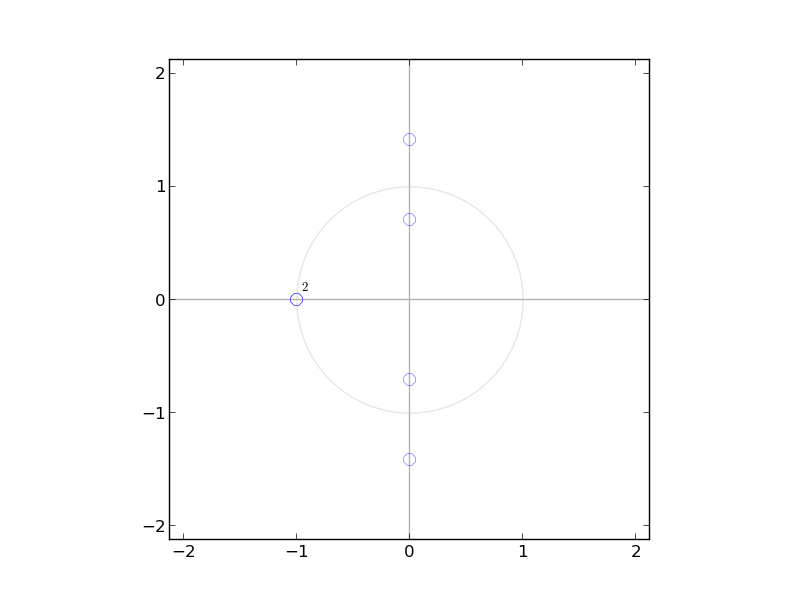
Pole Zero plots
Below are the pole zero plots for filter sizes of length 4
###Code
The code can be found at pyVision github repository
Files
- pyVision/pySignalProc/tutorial/wavelet5.py
References
- https://gist.github.com/endolith/4625838
- http://enc.tfode.com/Binomial-QMF
- http://web.njit.edu/~akansu/s1.htm
- http://www.bearcave.com/misl/misl_tech/wavelets/lifting/predict.html
- https://blancosilva.wordpress.com/teaching/mathematical-imaging/wavelets-in-sage/
- http://web.mit.edu/1.130/WebDocs/1.130/Software/Examples/example6.m
- http://fourier.eng.hmc.edu/e161/lectures/filterbank/node3.html
- http://enc.tfode.com/Binomial-QMF
- http://web.njit.edu/~akansu/s1.htm
- https://www.safaribooksonline.com/library/view/audio-signal-processing/9780471791478/ch006-sec004.html
- http://www.globalspec.com/reference/9046/348308/chapter-9-2-quadrature-mirror-filters-and-conjugate-quadrature-filters
- http://www.dsprelated.com/dspbooks/sasp/Conjugate_Quadrature_Filters_CQF.html
- http://www.raywenderlich.com/12065/how-to-create-a-simple-android-game
- https://gist.github.com/endolith/4625838
- http://enc.tfode.com/Binomial-QMF
- http://web.njit.edu/~akansu/s1.htm
- http://www.bearcave.com/misl/misl_tech/wavelets/lifting/predict.html
- https://blancosilva.wordpress.com/teaching/mathematical-imaging/wavelets-in-sage/
- http://web.mit.edu/1.130/WebDocs/1.130/Software/Examples/example6.m
- http://fourier.eng.hmc.edu/e161/lectures/filterbank/node3.html
- http://enc.tfode.com/Binomial-QMF
- http://web.njit.edu/~akansu/s1.htm