Approximation of Piecewise Polynomial Using Wavelets
29 Nov 2014Introduction
In this article we look at Approximation of Piecewise Polynomial Using Wavelets
Wavelet Approximation of polynomials
In many application,one needs to approximate a signal using scaling function ie using projection on $V_{m}$ subspace.
The support of a function is the set of points where the function is not zero-valued,The support of $\phi(t),\psi(t)$ which is defined over unit interval is 1
The basic analysis starts with considering a set of monomials ${1,t,t^2,\ldots,t^{k} }$ and asking the question till what degree $k$ can these be reproduced exactly using the scaling function.
Let us assume that $t^{p}$ can be represented exactly using the scaling function $t^{p} = \sum_{k} d_{k} \phi(t - k)$
Orthonormality of basis function impies
$d_{k} = \int t^{p} \phi(t -k ) dt$
To achieve this the scaling function should possess a certain properties which is dependent on the filter coefficients .
Restrictions on scaling and wavelet function
This assumption will impose certain restriction on the scaling and wavelet function
$\int t^{p} \psi(t) dt = \int \sum_{k} d_{k} \phi(t - k)\psi(t) dt = \sum_{k} d_{k} \int \phi(t - k)\psi(t) dt $
$\psi(t) ,\phi(t)$ are orthogonal ,meaning that $\phi(t)$ is capable of expressing polynomials upto degree $p$ exactly.
The projection of $t^{p} $ on $W_{m}$ subspace is 0. The projection of $t^{p} $ on $W_{m}$ subspace will not be zero only when it cannot be expressed completely by the scaling function.
if $p=0$,The condition implies
$\int \psi(t) dt =0$
Indicating that a constant function can always be expressed completely by scaling function.
we know that
$\psi(t) = \sum_{k} g[k] \phi(2t - k)$
$\phi(t) = \sum_{k} h[k] \phi(2t -k )$
We will use a result here which will be derived in later articles
$\int \psi(t) \phi(t) dt =0$ for this to hold true
$g[k]=(-1)^{N-k-1}h(N-k-1)$ and
$\psi(t) = \sum_{k} (-1)^{N-k-1}h(N-k-1) \phi(2t + k -N+1)$
for even N
$g[k]=(-1)^{k}h(N-k-1)$
$\int \sum_{k} (-1)^{N-k-1}h(N-k-1) \phi(2t + k -N+1) dt=0$
$\sum_{k} (-1)^{k} h(k) \int \phi(y) dy=0$
Vanishing Momemnt Constraint on wavelet filter coefficients
Zero order vanishing moment constraint $\sum_{k} (-1)^{k} h(k) =0$
pth order vanishing moment constraint $\sum_{k} (-1)^{k} k^{p}h(k) =0$
These vanishing moment constraint imposed on scaling and wavelet function help solve for the filter coefficients.
Projection of polynomials on subspace defined by Wavelets
Wavelet function $\psi(t)$ having N vanishing moments will kill polynomial upto degree $p-1$
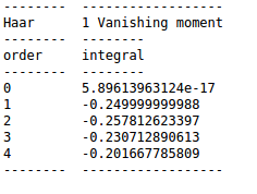
Let us look at a Haar wavelets function and projection of increasing order of polynomials on Haar wavelet basis.Haar wavelet has 1 vanishing moment.
Thus it can only kill polynomial of order 1 or constant function
Daubechies -2 wavelet has vanishing moment of 2 ,Thus it can kill polynomial upto degree of 2 A constant and linear function.

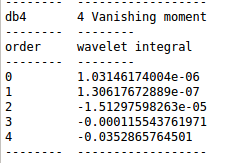
Daubechies -4 has vanishing moment of 4 ,Thus it can kill polynomials upto a degree of 3
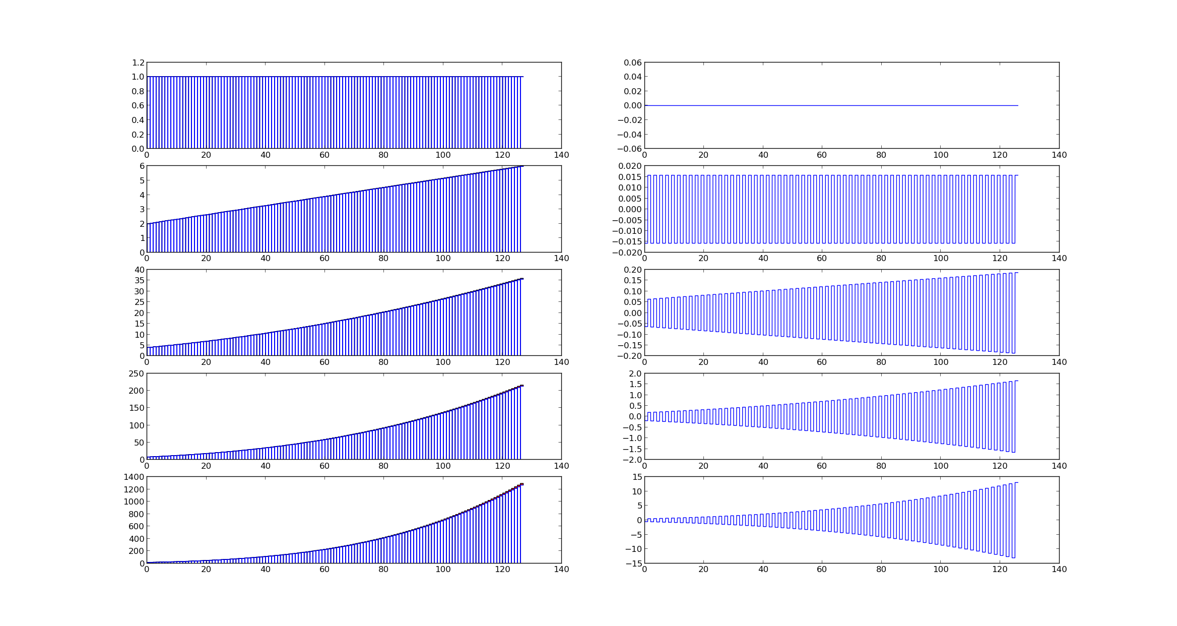
What this means is that projection on $W_{o}$ subspace is zero.Wavelet coefficients will have low magnitude .Typically threshold should be less than $1^{-7}$.This will imply signal can be reconstructed from the projection on $V_{0}$ subspace to a great degree of accuracy
We can see the projection on the $V_{0}$ and $W_{0}$ subspace in the below figures
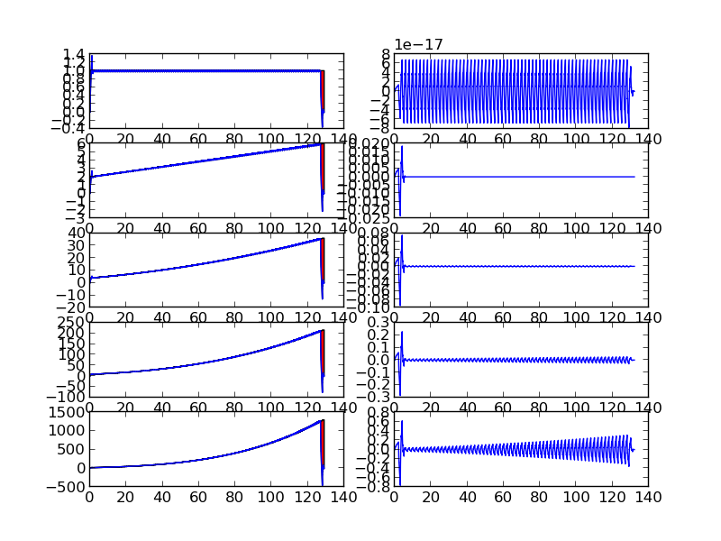
Projection of Piecewise polynomials on subspace defined by Wavelets
It is important to note that it is sufficient that function behaves like a polynomial of degree $k$ over support of function for it to be approximated by scaling function.
Below figures show piecewise polynomials and projection on $V_{0}$ and $W_{0}$ subspace
We can see that piece-wise polynomials of degree $p$ within the support of wavelet functions with vanishing moment $p$ have zero wavelet coefficients except at points of discontinuity
Code
The function plotwaveletProjection plots the projection of signal onto the $V_{m}$ and $W_{m}$ subspace
def plotWaveletProjection(x,coeff,w,level=1,mode=0):
""" function plots the projection of signal on the scaling and wavelet functions subspace
Parameters
-----------
x : numpy-array,
The input signal
coeff : numpy=-array
The wavelet or scaling coefficient
w : pywt.Wavelet
wavelet object
level : integer
decomposition level
mode : integer
scaling or wavelet coefficient
Returns
--------
out : numpy-tuple
(time,reconstruction,signal)
"""
#generate the scaling and wavelet functions
s1,w1,t2=w.wavefun(level=20)
#setup 1D interpolating function for scaling and wavelet functions
wavelet=interpolate.interp1d(t2, w1)
scaling=interpolate.interp1d(t2, s1)
time=[]
sig=[]
s1=np.array(s1,float)
#compute the dydactic scale
l=2**level
#find the support
end1=math.floor(t2[len(t2)-1])
d=abs(float(len(coeff))*float(l)-len(x))
d=int(d)
#range over each element of coefficient
for i in range(len(coeff)-1):
#define the interpolation points
t=np.linspace(l*i,l*i+l*end1,l*end1*(len(x)));
t1=np.linspace(0,end1,end1*(len(x))*l);
#multiply the coefficient value with scaling or interpolation function
if mode==0:
val=coeff[i]*scaling(t1)
else:
val=coeff[i]*wavelet(t1)
ratio=end1
#compute the translation
inc=len(t)/ratio
if i==0:
sig=np.append(sig,val)
time=np.append(time,t)
else:
#compute the incremental sum of signals
v1=val[0:len(t)-inc]
if inc < len(t):
v2=val[len(t)-inc:len(t)]
sig[i*inc:i*inc+len(t)]=sig[i*inc:i*inc+len(t)]+v1
sig=np.append(sig,v2)
time=np.append(time,np.linspace(l*i+l*end1-l,l*i+l*end1,inc))
else:
sig=np.append(sig,val)
time=np.append(time,t)
#flatten the arrays
sig=np.array(sig).flatten()
time=np.array(time).flatten().ravel()
#scale the values due to didactic decomposition
sig=sig/(math.sqrt(2)**level)
#upsamples the value of signal
x=np.repeat(x,len(sig)/len(x))
#return the signals,which can be plotted
return time,sig,x
A class called “PiecewiseContinuous “ encapsulates all the methods that define a piece-wise continuous function.The function is modified version of the function from sagemath library
 # piecewise function
def f1(x):return 10
def f2(x):return 5*x
def f3(x):return 2*(x)**2
def f4(x):return (x)**3+(x)**2
def f5(x):return 20*((x)**5)

f = Piecewise([[(0,1),f5],[(1,2),f4],[(2,3),f3],[(3,4),f2],[(4,5),f1]])

f(1) will give the value the value of piecewise function at 1
All the plots and results presented in the article can be generated by running the wavelet4.py files
Files
The code can be found in pyVision github repository
- pyVision/pySignalProc/tutorials/wavelet4.py
- pyVision/pySignalProc/wavelet/pywtUtils.py