Haar Wavelets

Introduction

In this article we will look at basic introduction to wavelets using Haar wavelets

Haar Wavelets

Lets take the consider a family of wavelets called Haar Wavelets.The Haar wavelet are simplest form of wavelets.

The idea of wavelets is to express contininuous singal linear combination of wavelet function. Let is first see what Haar wavelets look like

Piece-wise constant approximation

The idea of piecewise constant approximation is to represent signal in duration of interval T by a constant. One of measures that can be used is to represent the signal using mean value of signal over the interval.

Let consider a continuous time signal $x(t)$ and look at piecewise constant approximation of the signal.

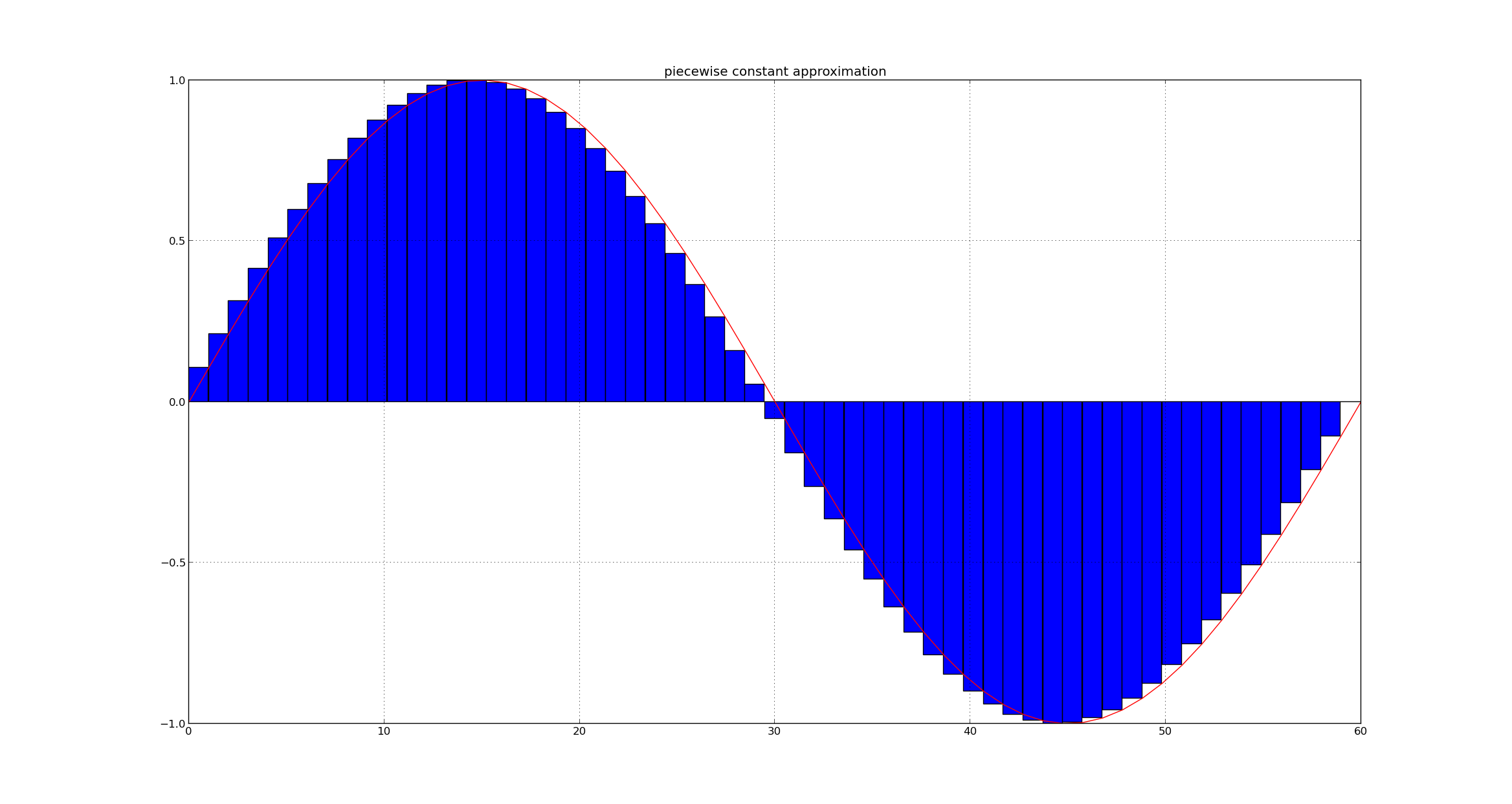
We will perform picewise contant approximation of signal over interval length of $T=8$ $\displaystyle x_{T}(t)= \frac{1}{T}\int_{T} x(t) dt $

We can see this in the below figure

Let $\phi(t)$ represent a unit step function,The approximated signal can also be expressed as $x_{a}(t) = \sum_{i} x_{T}(t) \phi(t - iT)$

$\psi(t - iT)$ represents constant integral translations of the unit step function

Thus any arbitrary function can be expressed can be expressed as linear combination piecewise constant integer translates of function $\phi(t)$

Basic function

The set of function ${\phi(t)}$ and its interger translates are said to span a linear space $\mathcal{F}$ if any function in the space $\mathcal{F}$ can be expressed as linear combination of this set.

Let $V_{o}$ represent such a space where any function can be expressed as linear combination of ${\phi(t)}$ and its interger translates.Any function in $V_{o}$ can be expressed as $\sum_{n \in \mathcal{Z}} C_{n} \phi(t- n)$

$V_{0}$ is a space of piecewise constant function on interval of size $T$

The set of function ${\phi(t)}$ are called the basis of space $\mathcal{F}$

we can also see that $\int \phi(t-kT) \phi(t-iT)=0,i\neq k$ and $\int \phi(t-kT) \phi(t-iT)=1,i= k$

The basics also forms a orthonormal set

Subspaces of piecewise constant functions

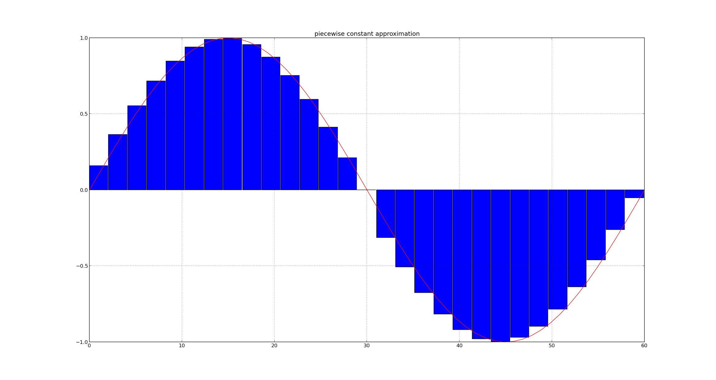
Now let us consider piecewise constant approximation over interval length of $T/2=4$ where $s=1/2$

This can be seen in below figure

$x_{s,a}(t) = \sum_{i} x_{T}(t) \phi_{s}(t - iT)$

and $\phi_{s}(t) = \phi(\frac{t}{s})$

$x_{s,a}(t) = \sum_{i} x_{T}(t) \phi(\frac{t - iT}{s})$

Thus function is expressed as linear combination of integral translates of scaled version of function $\phi(t)$ Let $V_{1}$ denote the linear space spanned by $\phi(\frac{t}{s})=\phi(2t)$ and its integer translates

$x_{s=2,a}(t) = \sum_{n} x_{T}(t) \phi(\frac{t}{s} - n)$

Any space $V_{m}(t)$ can be similarily constructed

$V_{m} = span_{n \in \mathcal{Z}} { \phi(\frac{t}{s} - n)}$

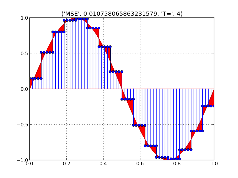
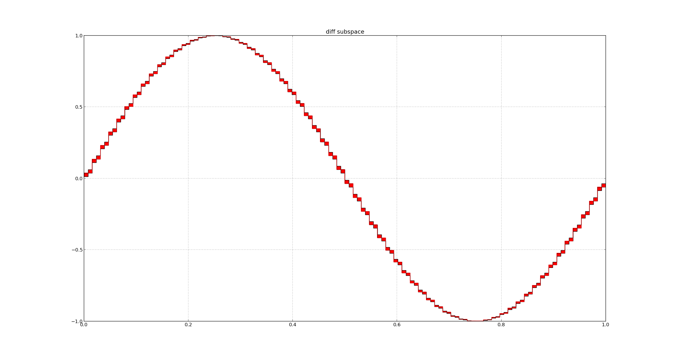
Lets take a signal $x(t)$ and its projection in subspace $V_{0}$ and $V_{1}$ in the present example $T=8$

We can see as we take smaller intervals or projection of subspace $V_{1},V_{2},\ldots V_{m}$ we get better approximation of the signal

we plot both the projection and red region indicates the difference between the projection.

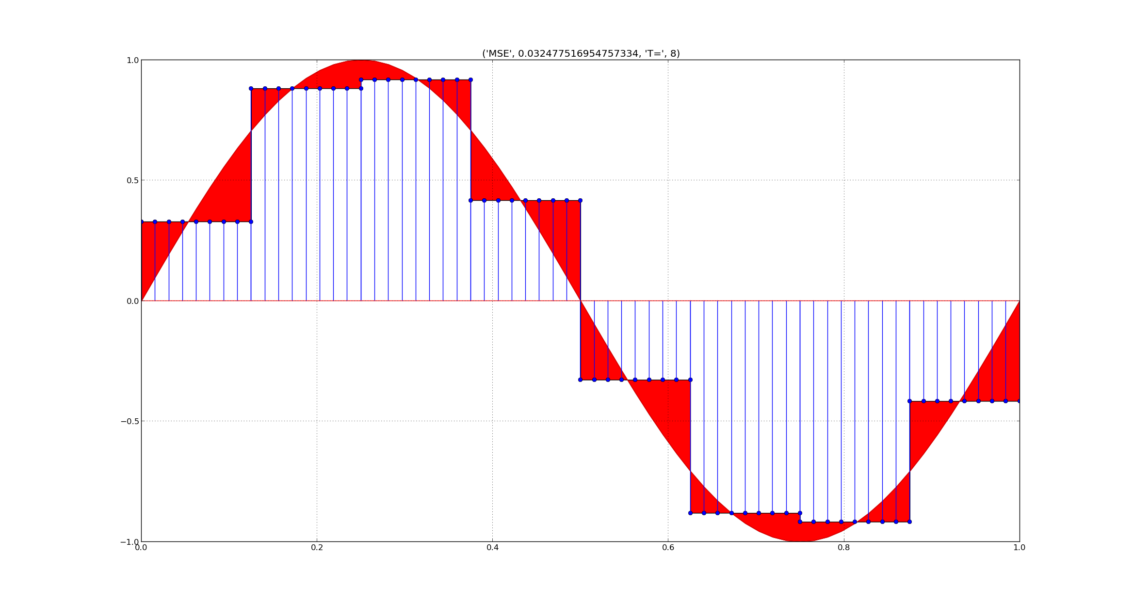
we can see that the mean square error reduces as we take projection of higher subspaces As we take smaller and smaller intervals,we can better approximate the continuous time signal

we can see that X_{T}(t) is a sequence and equivalence between $x(t)$ and sequence $X_{T}(t)$ we will write $X_{T}(t)$ as $x[n]$ which are the components of projection along orthonornal basis ${ \phi(t)}$

$x_{s,a}(t) = \sum_{n} x[n]\phi(\frac{t}{s} - n)$

Thus $x(t) \in \mathcal{L}_{2}(\mathcal{R})$ implies $x[n] \in l_{p}(\mathcal{Z})$ where $l_{p}(\mathcal{Z})$ is linear space of set of integers

Ladder of subspaces

we can also see that $x_{s=1,a}(t)$ can also be expressed as a linear combination of $\phi(\frac{t}{s} )$ and its integral translates.

Thus linear space $V_{0}$ is also spanned by $\phi(\frac{t}{s} )$ and its integer translates. It can also been seen that $V_{o}$ is a subspace of $V_{1}$.

where $s=2^{M}$ for case we take didactic scale of $T,T/2,T/4 \ldots $

$V_{m} = span_{n \in \mathcal{Z}} { \phi(st - n)}$

and $\ldots \subset V_{-1} \subset V_{o} \subset V_{1} \subset V_{2} \ldots \subset V_{m} \ldots \mathcal{L}_{2}(\mathcal{R})$

Thus there exits a ladder of subspaces which allow us to represent the signal using appriopriate basis at desired resolution

In wavelet terminalogy $\phi(t)$ is called a scaling function and basis of ladder of subspaces are defined in terms of scaled version of scaling function

Wavelet function

Let us consider the subspaces $V_{0}$ and $V_{1}$ and observe the difference between the signals approximated by these two subspaces

We can observe a pattern here ,The shape of the difference function in all the intervals is the same

Let us denote the subspace spanned by this difference as $W_{0}$

$V_{1} = V_{0} + W_{0}$

Let’s look at the reason why this is so

$x_{1,a}(t) = \sum_{n} x[n]\phi({t} - n)$

$x_{2,a}(t) = \sum_{n} z[n]\phi(2t - n)$

where $\phi(t)$ is defined over interval T and $\phi(2t)$ is defined over interval of T/2

Let us look at single interval over T and projection $V_{0},V_{1}$

we can express the these measures as

$\displaystyle x_{1,\frac{T}{2}}(t)= \frac{2}{T}\int_{0}^{\frac{T}{2}} x(t)dt =\frac{2}{T}\int x(t) \phi(2t)dt$

$\displaystyle x_{2,\frac{T}{2}}(t)= \frac{2}{T}\int_{\frac{T}{2}}^{T} x(t)dt =\frac{2}{T}\int x(t) \phi(2t-\frac{T}{2})$

$\phi(st) = 1 $ for $t\in [0,\frac{T}{s}]$

Now we need to relate $x_{T}(t)$ piecewise constant approximation over the entire duration T with measures $x_{1,\frac{T}{2}}(t),x_{2,\frac{T}{2}}(t)$ which are piecewise constant approximation over duration $\frac{T}{2}$ of the signal.

$\displaystyle x_{T}(t) = \frac{1}{2} [ x_{1,\frac{T}{2}}(t) +x_{2,\frac{T}{2}}(t) ]$

$\displaystyle x_{T}(t) = \frac{1}{2} \sum_{i} x_{i,\frac{T}{2}}(t) $

$\displaystyle x_{T}(t) = \frac{1}{T} [ \int x(t)\phi(2t)dt +\int x(t)\phi(2t-\frac{T}{2})dt ]$

$\displaystyle x_{T}(t) = \frac{1}{2^N} \sum_{i\in 2^N} x_{i,\frac{T}{2^N}}(t) $

Let us look at difference between approximation in the projection on $V_0$ and $V_{1}$ over interval of $[0,\frac{T}{2}$ and $[\frac{T}{2},T]$

$e_{0}(t) = x_{1,\frac{T}{2}}(t) - x_{1,T}(t) $

$e_{0}(t) =\frac{2}{T}\int_{0}^{\frac{T}{2}} x(t) dt -\frac{1}{T} \int_{0}^{T} x(t) dt$

$e_{0}(t) =\frac{1}{T}\int_{0}^{\frac{T}{2}} x(t) dt -\frac{1}{T} \int_{\frac{T}{2}}^{T} x(t) dt$

Similarily $e_{1}(t) =\frac{2}{T}\int_{\frac{T}{2}}^{T} x(t) dt -\frac{1}{T} \int_{0}^{T} x(t) dt$

$e_{1}(t) =\frac{1}{T}\int_{\frac{T}{2}}^{T} x(t) dt -\frac{1}{T} \int_{0}^{\frac{T}{2}} x(t) dt$

the error over interval of T can be written as

$e(t) = A \phi(2t) - A \phi(2t -\frac{T}{2})$

$\psi(t) = \phi(2t ) - \phi (2t -\frac{T}{2})$

$e(t) = A \psi(t)$

This is exactly the shape of function we observed in each interval

This is called as wavelet function.

The wavelet function for the basis of subspace $W_{0}$. we can also see that basis $\psi(t)$ can be expressed as linear combination of $\phi(t)$.

Thus $W_{0} \subset V_{1}$ and Thus $V_{0} \subset V_{1}$

The coefficients of projection on $V_{1}$ subspace can be computed using the wavelet function

$V_{1} = V_{0} + W_{0}$

$V_{1} = V_{-1} + W_{-1} + W_{0}$

$V_{1} = V_{-2} +W_{-2} + W_{-1} + W_{0}$

$V_{0} $ is subspace with $\phi(t)$ defined over unit interval.

Haar Wavelet

The wavelet and scaling function of Haar Wavelet is as below

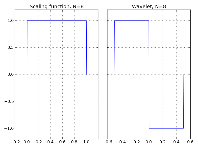
They can be expressed as $ [ \frac{1}{\sqrt2} ,\frac{1}{\sqrt2} ] $ $ [\frac{1}{\sqrt2},-\frac{1}{\sqrt2} ] $

Signal Decomposition Using Wavelets

Where $V_{1}$ can be considered as sampled sequence,Now we can express this signal in terms of scaling and wavelet functions.

Let $x[n]$ represent the discrete time sequence .This can be considered as projection coefficients on the $V_{0}$ subspace.

Thus we can represent the projection on $V_{-1}$ subspace as $y[n]=\frac{1}{\sqrt2}\frac{1}{2} x[2n]+x[2n+1]$

we can represent the project on the $W_{0}$ subspace as $y[n]=\frac{1}{\sqrt2} \frac{1}{2} x[2n]-x[2n+1]$

let us consider a dummy input sequence $x=[1,1,1,1,1,1]$

$V_{-1}=[ 1.41421356 , 1.41421356, 1.41421356]$

$W_{0}=[ 0., 0, 0.]$

Now let us look at projection on subspace $V_{-2},W_{-1}$

$V_{-2}=[ 2., 2.]$

$W_{-1}=[ 0. , 0.]$

The process of expressing a signal in terms of the wavelet basis is called signal decomposition

Code

The code for generating the plot can be found in the github pyVision repository

• pyVision/pySignalProc/tutorial/wavelet1.py

Download the entire repository and run the wavelet1.py files

The code uses pyWavelets python package.This needs to be installed before running the code.