Time Delay Estimation Techniques - Part 1
13 Oct 2014Introduction
In this article we will look at signal processing techniques for time delay estimation.
Background
Time delay estimation has been a research topic of significant practical importance in many fields like radar, sonar, seismology, geophysics, ultrasonic’s, hands-free communications,Doppler positioning systems etc and is of fundamental importance in a variety of signal-processing applications.
The problem boils down to computing the location of a digitized “signature” waveform residing within a larger time-slice.
Let $s(n)$ be the sound source signal. Let us consider two spatially separated sensors and $x_{1}(t)$ and $x_{2}(t)$ be result of propagation of $s(t)$ through different paths to reach the respective sensors.
A simple propagation model is that the signals just encounter attenuation and delay and are corrupted by additive noise
$x_{i}(t) = a_{i} s(t- \tau_{i}) + b_{i}(t)$
where ,
$b_{i}(t)$ is the additive noise uncorrelated with the signal
We make a assumption that the distance from the sensors to the source is very large compared to the spatial separation between the sensors.Thus signal $s(t)$ received by both the receivers is the same,there is no significant change in the signal as it travels thorough different paths to reach the spatially separated sensors.
Cross-correlation
One of the simplest method of time delay estimation is cross-correlation . The cross-correlation of two signals is a measure of similarity between the two sequences. The cross-correlation function is maximized when both the signals have significant overlap.
$R_{xy}(k) = \sum_{i} {x(i) y(i+k)} = x[n]*y[-n]$
Compute maximum absolute value of the correlation function to estimate the lag.
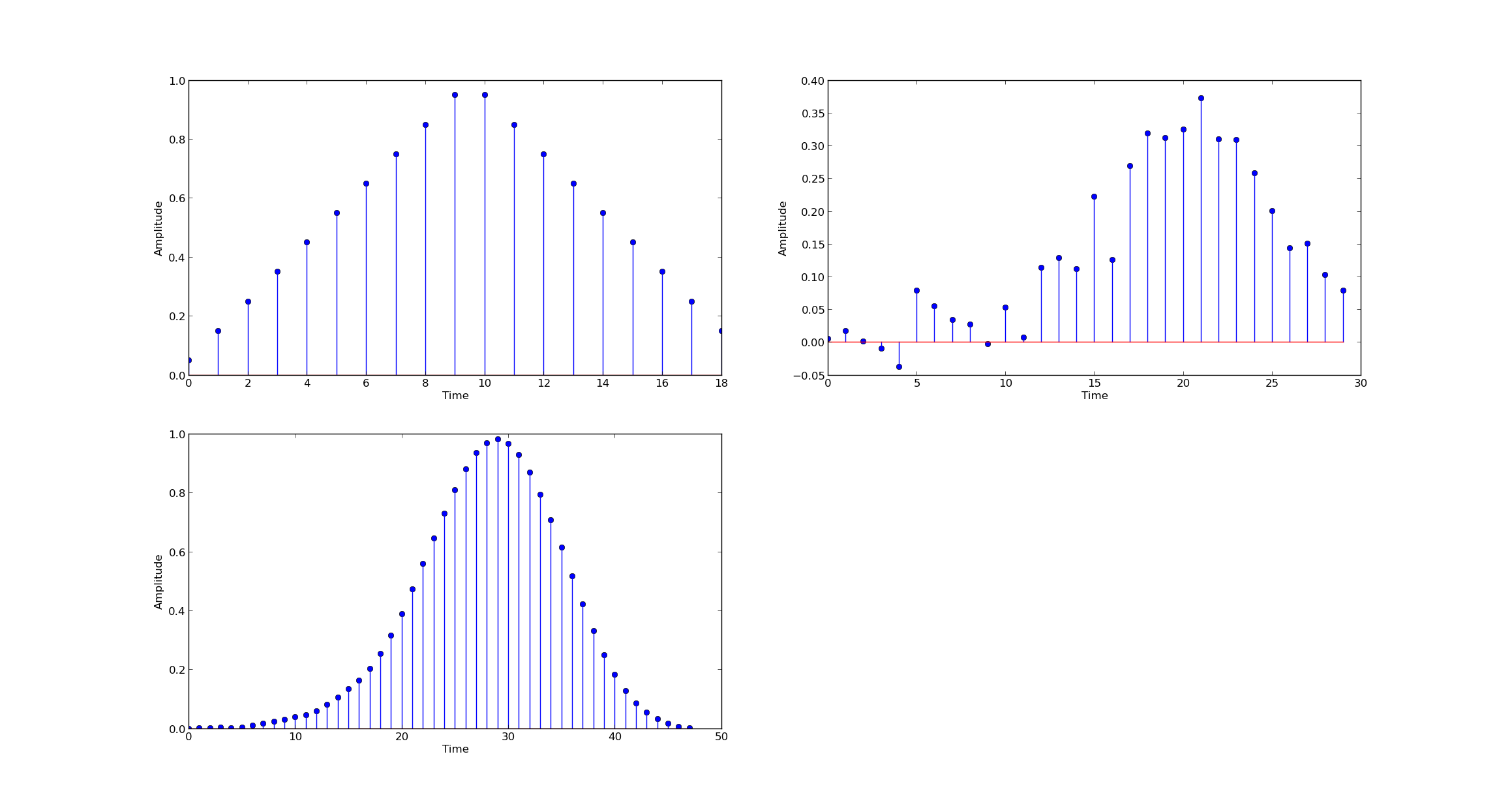
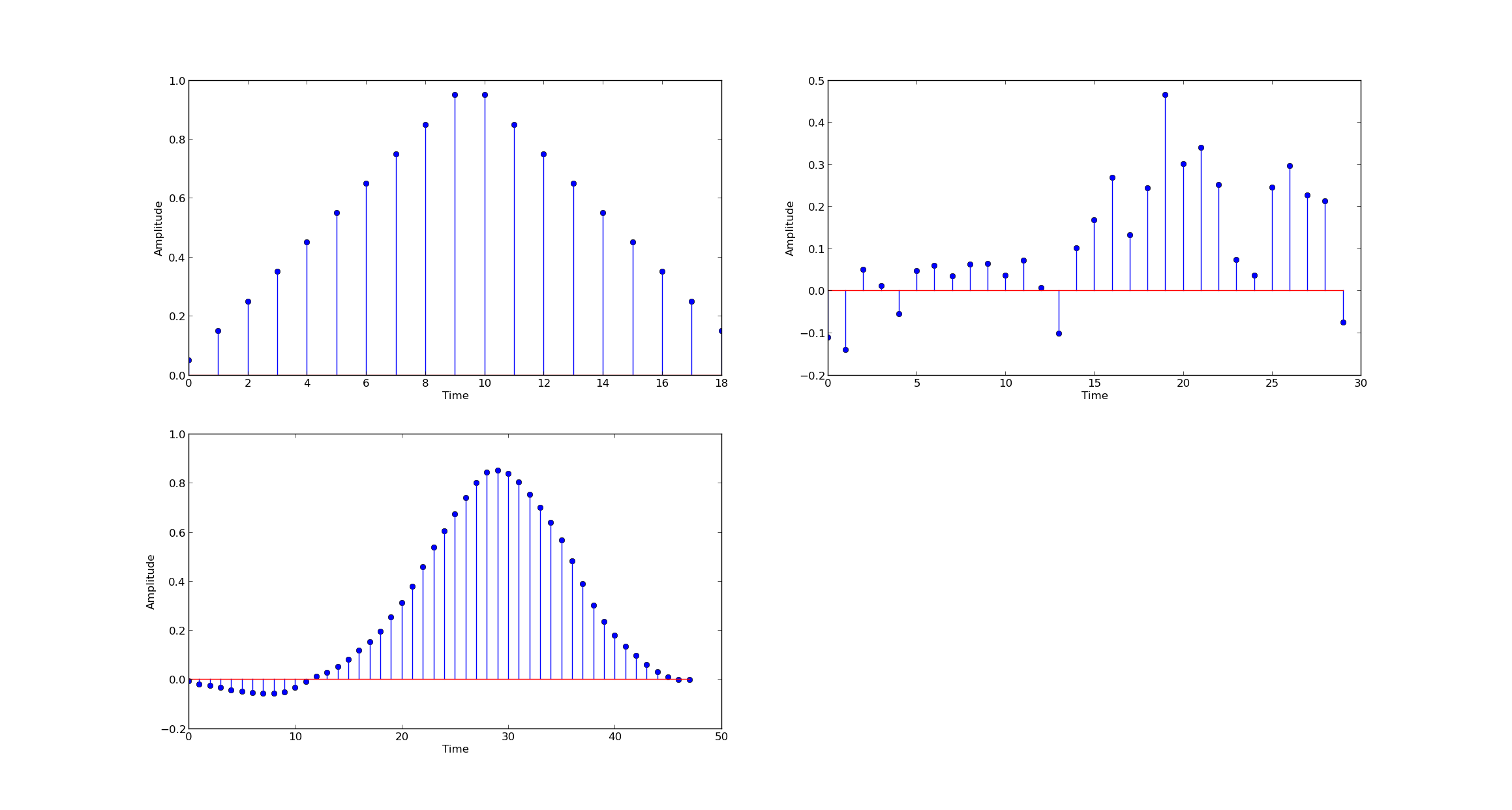
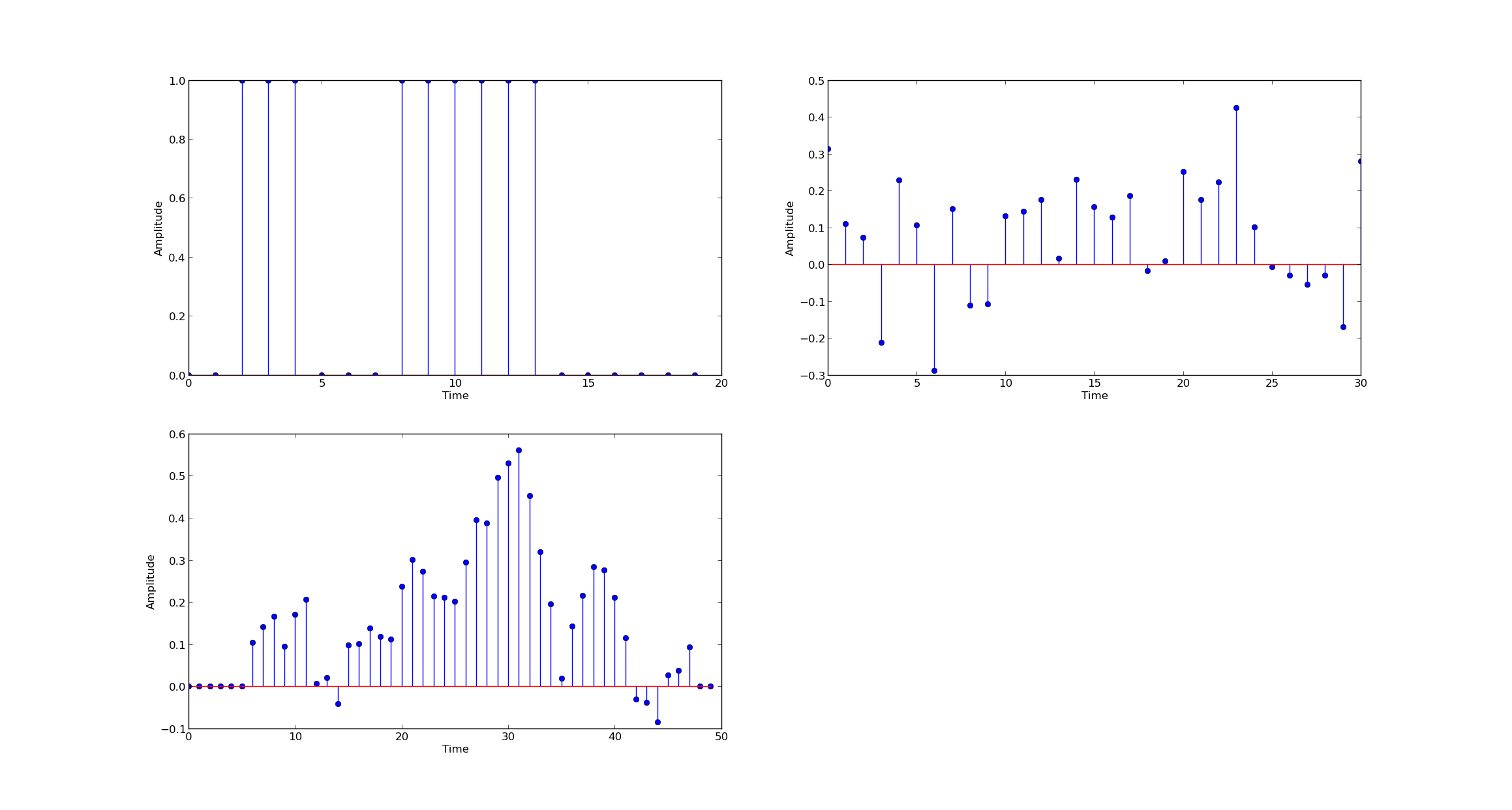
To test the results we create create two sequences,one a delayed version of another. We add white noise to the delayed sequence and use sample correlation to detect the lag. while performing correlation we normalize the signals,so that correlation measure is bounded between [0,1]
Now we increase the noise to try to get estimate of noise co-variance at which this technique fails. we run the experiment 100 times and estimate the number of times we get the proper answer.
Testing with Different Additive Noise Covariance
 *********** Information ************
time delay :  10
Noise : 0.1
SNR 15.4390474505
Correct  98  Incorrect  3
mean  9.90099009901 Std  1.0000490136
We see that we are always correct,when the noise levels are low or SNR is high
 *********** Information ************
time delay :  10
Noise : 0.3
SNR 5.89662235611
Correct  48  Incorrect  53
mean  9.79207920792 Std  1.2767287382
The SNR has dropped to about 6db and error in estimation is about 50%. The accuracy is linearly related with the SNR
 *********** Information ************
time delay :  10
Noise : 0.5
SNR 1.45964736379
Correct  36  Incorrect  65
mean  9.80198019802 Std  1.57969668714
At 2 db SNR we can see the variance of estimated time delay increasing with rising noise levels.
We can see in the auto-correlation plot the difference between the peak and its neighbors is not significant and depending on the random noise levels introduced,we may not always get the right answer.
As noise increases,we can see variance in the estimated time delay increases and error in estimation also increases.As the level of noise increases, the uncertainty in the time-delay estimate increases
We need a reliable time delay estimator in presence of additive noise.
If is always difficult to estimate the time delays for a base-band signal illustrated above.The due to the noise,we are not reliably able to estimate the delay corresponding to the maximal overlap between the noisy and ideal signal.
def delay(signal,N):
    """ function introduces a delay of N samples

    Parameters
    -----------
    signal : numpy-array,
             The input signal

    N      : integer
             delay

    Returns
    --------
    out : numpy-array
          delayed signal

    """
    d=numpy.zeros((1,N+1));
    signal=numpy.append(d,signal)
    return signal;

def addNoise(s,variance):
    """ function add additive white gaussian noise to the input signal

    Parameters
    -----------
    s : numpy-array,
             The input signal

    N      : float
             noise covariance

    Returns
    --------
    out : numpy-array
          noisy signal

    """
    noise = np.random.normal(0,variance,len(s))
    s=s+noise;
    return s;


if __name__ == "__main__":

        Fs=1000;

        mode=0
        if mode==0:
            x = triang(20);
            x2=x;

		......

        tdelay=10;
        varnoise=0.001;
        loop=1000


        #delay the signal
        dx=delay(x,tdelay);
        result=numpy.zeros((1,loop));
        for i in range(loop):
            s=dx;
            #add noise
            s=addNoise(s,varnoise);

            #normalize the signals
            s=s/np.linalg.norm(s);
            x1=x2/np.linalg.norm(x2);

            unfiltered_signal=s;

            r=numpy.correlate(s,x1,mode="full")
            arg=np.argmax(r)
            result[0,i]=abs(arg-len(x))

		#plot the results
	    c=np.sum(result==tdelay)
        ic=np.sum(result!=tdelay)
        #10*np.log(np.sum(np.abs(x*x))/
        print " *********** Information ************ "
        print 'time delay : ',tdelay
        print 'Noise :',varnoise
        print "SNR",10*np.log(np.mean(abs(x*x))/(varnoise*varnoise))/np.log(10);
        print "Correct ",str(c)," Incorrect ",str(ic)
        print "mean ",np.mean(result),"Std ",np.std(result)
        print result
        plt.figure(1)
        subplot(2,2,1)
        plt.plot(range(len(x)),x)
        xlabel('Time')
        ylabel('Amplitude')


        subplot(2,2,2)
        plt.plot(range(len(unfiltered_signal)),unfiltered_signal)
        xlabel('Time')
        ylabel('Amplitude')

        subplot(2,2,3)
        plt.plot(range(len(r)),r)
        xlabel('Time')
        ylabel('Amplitude')
Rectangular Pulse signals
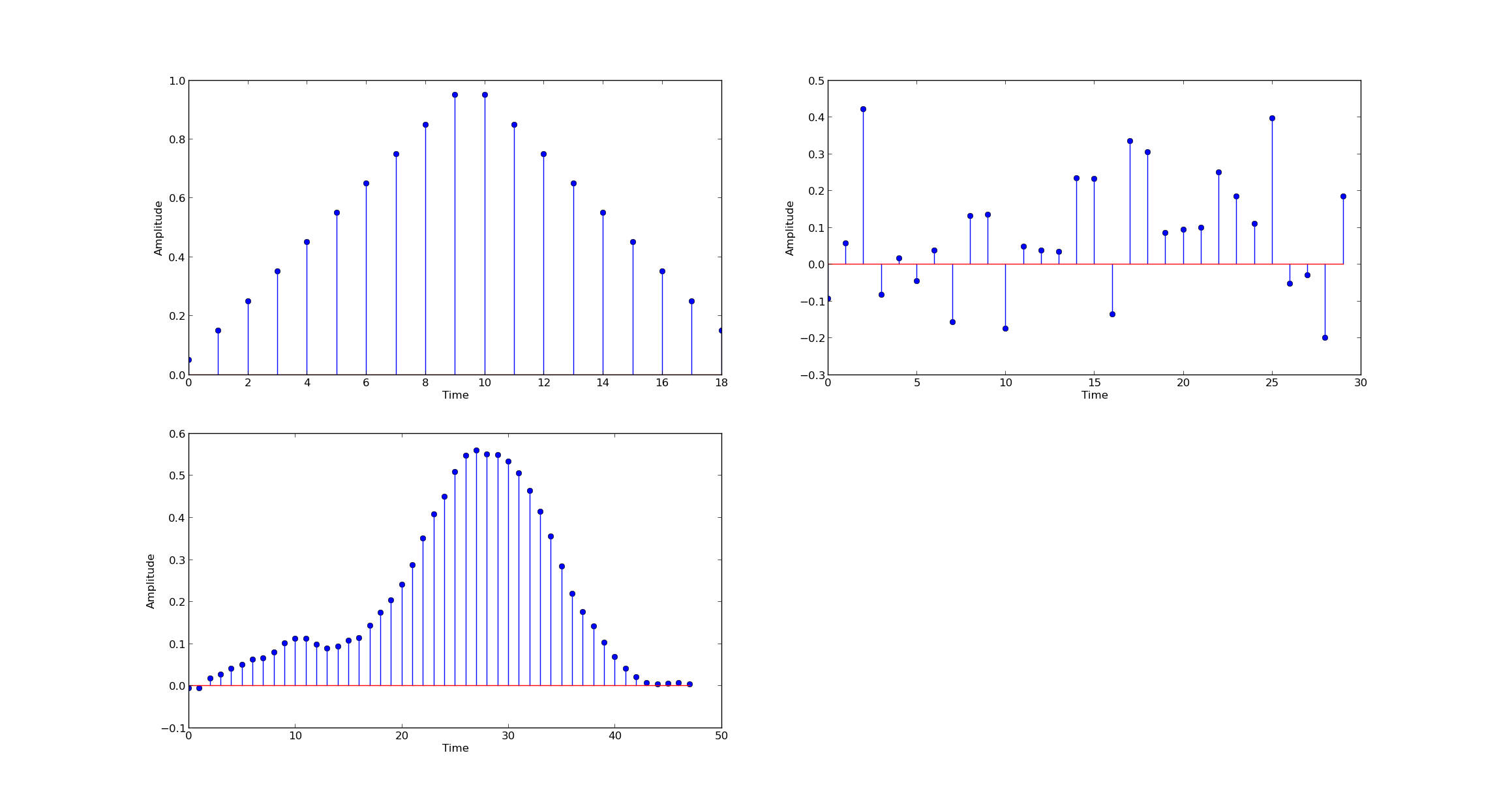
Let us look at the results for a different signal in the form of a rectangular pulse . we will consider the wave of same duration 30.
 *********** Information ************
time delay :  10
Noise : 0.5
SNR 0.791812460476
Correct  86  Incorrect  15
mean  9.92079207921 Std  1.11411438271
we see that signal has a lower SNR,but accuracy and estimated time delay variance is lower.
 Thus the type of pulse we use has a impact on the accuracy of auto-correlation function.
def rectangular(N,start,end):
        """ fuction generates a rectangular pulse

        Parameters
        ---------
        N : integer
            length of signal

        start,end: integer
                starting and ending index of pulse

        """
        x = np.zeros((1,N))
        x[:,start:end]=1;
        x=x.flatten();
        return x;
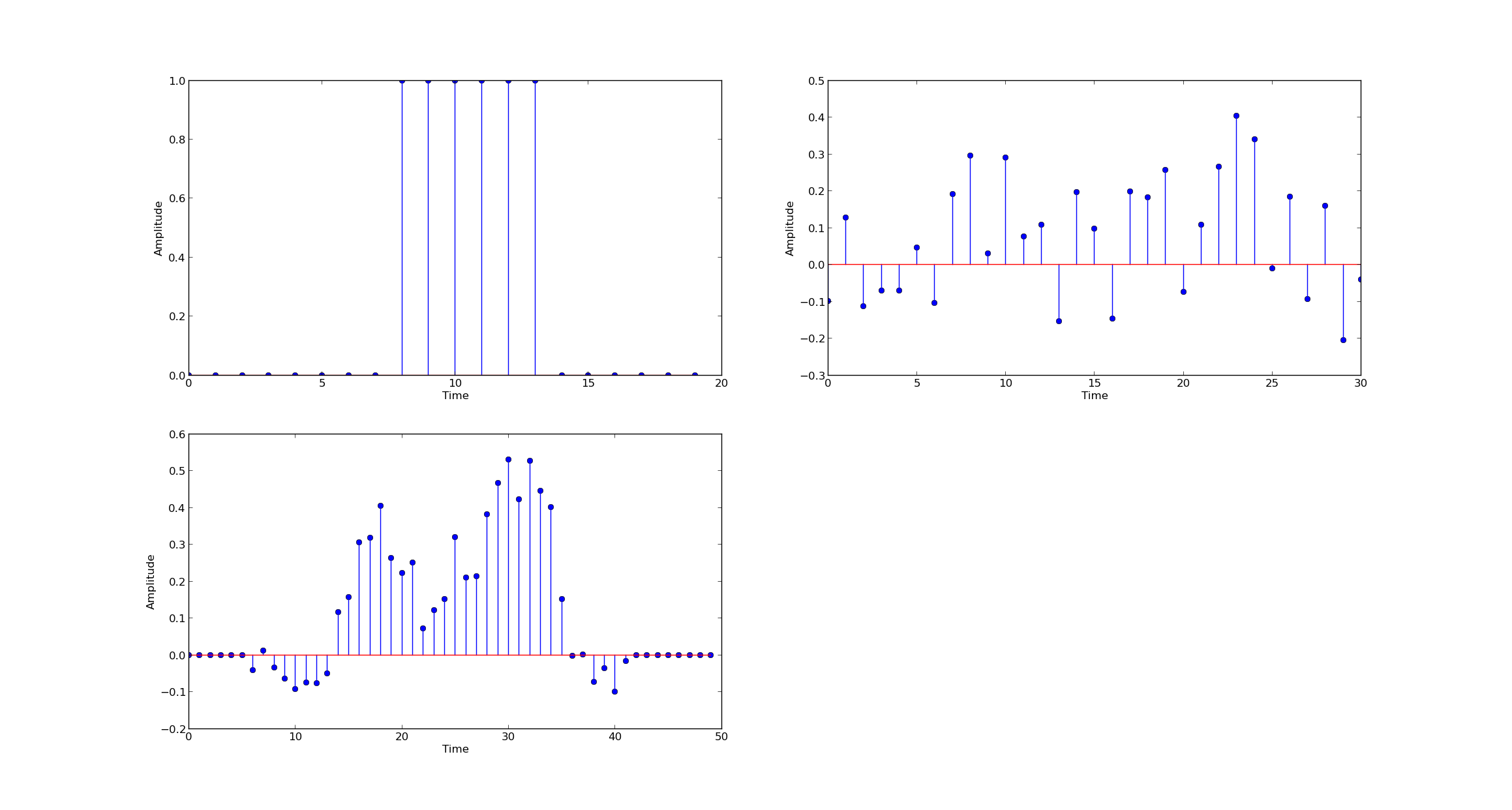
Coded Pulses
Broadband techniques have a sequence of code pulses that increase the accuracy of time delay estimation in the presence of noise.
time delay :  10
Noise : 0.5
SNR 2.55272505103
Correct  95  Incorrect  6
mean  9.93069306931 Std  1.01725144864
x=rectangular(20,8,14)+rectangular(20,2,5)
But most of the time we do not have control of the source pulse.
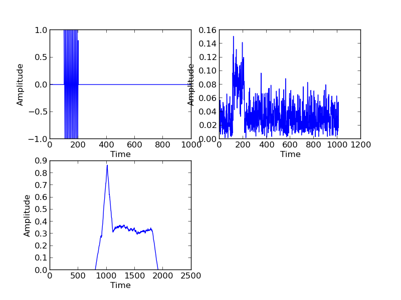
In the remainder of the article we will assume that it is a rectangular pulse of duration 1000 with impulse of duration 50 starting at 100.
time delay :  10
Noise : 0.5
SNR -6.98970004336
Correct  856  Incorrect  144
mean  9.991 Std  0.561176442841
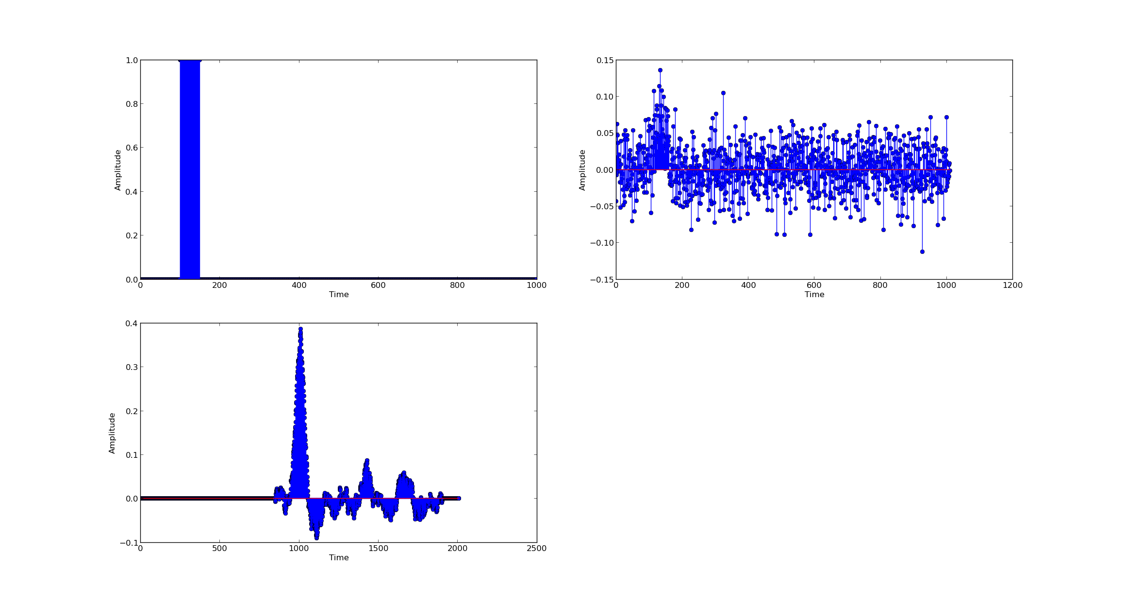
x=rectangular(1000,100,150)
Now given source signal,we need to see if we can do better in the presence of additive noise atleast.In real life situations there will be a host of other distortions and effects which will increase the estimation errors apart from noise.
For pulses like the ones observed above,noise is a dominant factor,signal energy is low compared to noise energy.
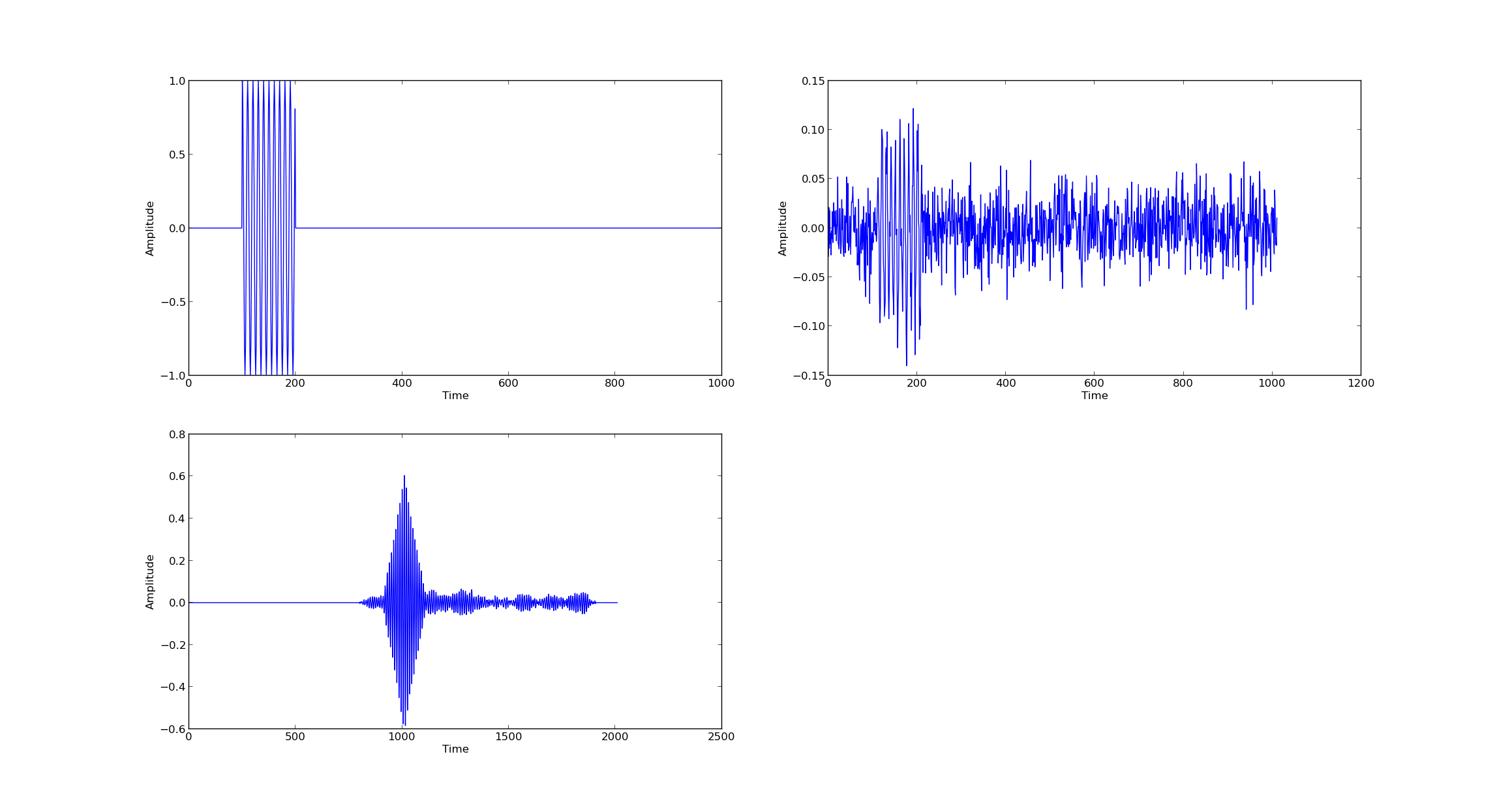
Modulated Pulses
Often the pulses are modulated by sinusoidal waves for longer range transmissions. </pre> time delay : 10 Noise : 0.5 SNR -6.98970004336 Correct 988 Incorrect 12 mean 10.004 Std 0.109471457467 Actual time delay 10 </pre>
def sinepulse(N,start,end,f,Fs=1000,tau=0):
        """ function generates modulated rectangular pulse

        Parameters
        ---------
        N : integer
            length of signal

        start,end: integer
                starting and ending index of pulse

        f   : integer
              modulated carrier freuency

        Fs  : integer
              Sampling freuency

        tau : integer
              carrier phase delay in samples.

        Returns
        --------
        out : numpy-array
              modulated rectangular  signal

        """
        x = np.zeros((1,N))
        t=np.asarray(range(0,end-start));
        x[:,start:end]=np.cos(2*np.pi*f*(t+tau)/Fs);

        return x.flatten();
Carrier Synchronization Issues
we can synchronize exactly with the carrier ,then like broadband techniques we can achieve a significantly enhanced SNR. However synchronizations are never possible.
we introduce a phase delay of 1 sample to check the effect of carrier phase errors
*********** Information ************
time delay :  10
Noise : 0.3
SNR -2.55272505103
Correct  2  Incorrect  998
mean  229.036 Std  244.973840857
In such cases another approach might be to use rectangular envelope but in the present case that also does not seem to help
 *********** Information ************
time delay :  10
Noise : 0.3
SNR -2.55272505103
Correct  0  Incorrect  1000
mean  325.336 Std  272.058543523
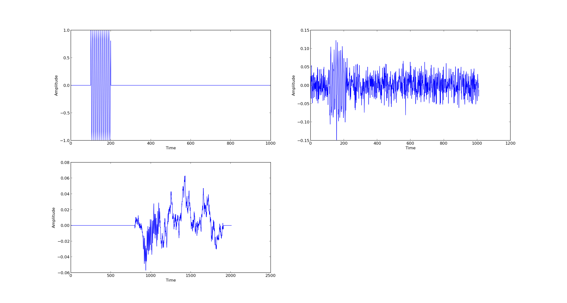
Envelope Detection
We perform envelope detection on the signal and then apply correlation. This improves the situation considerably
 *********** Information ************
time delay :  10
Noise : 0.3
SNR -2.55272505103
Correct  661  Incorrect  339
mean  9.746 Std  0.793400277288
            if mode==5 or mode ==6 or mode==7:
                s=abs(scipy.signal.hilbert(s))
Filtering
If we known the carrier frequency ,we can filter the noise outside the signal bandwidth before performing the correlation operation.
For the remaining examples we consider signal with carrier frequency of 1KHz and Sampling rate of 5Khz. The reason for that is explained below
Let us first look at the frequency characteristics of the rectangular pulse
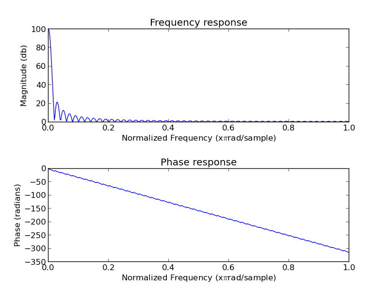
The sharp transition at the edges of the rectangular pulse give rise to high frequency components. Thus while filtering we need to take these into account,else we may end up distorting the edge leading to errors in time delay estimation.
The width of the mainlobe in frequency domain is inversely proportional to width of rectangular pulse in the time domain.Thus a wider pulse in the time domain will provide higher spectral compression in the frequency domain.
we can see that main lobe of the rectangular pulse would have normalize freuency of 0.05 Few of the side lobes also contain significant information.
def plotFrequency(b,a=1):
    """ the function plots the frequency and phase response """
    w,h = signal.freqz(b,a)
    h_dB = abs(h);#20 * np.log(abs(h))/np.log(10)
    subplot(211)
    plot(w/max(w),h_dB)
    #plt.ylim(-150, 5)
    ylabel('Magnitude (db)')
    xlabel(r'Normalized Frequency (x$\pi$rad/sample)')
    title(r'Frequency response')
    subplot(212)
    h_Phase = np.unwrap(np.arctan2(np.imag(h),np.real(h)))
    plot(w/max(w),h_Phase)
    ylabel('Phase (radians)')
    xlabel(r'Normalized Frequency (x$\pi$rad/sample)')
    title(r'Phase response')
    plt.subplots_adjust(hspace=0.5)
We try with a normalized frequency components of 0.05 which contains around 3 adjacent side-lobes
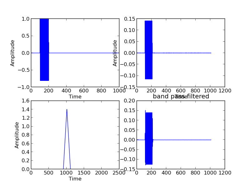
we can see that the signal has been attenuated near the edges.Thus the distortion in the region where the pulse starts will lead to ambiguity of time delay computation.
Thus we need to consider the freuency components to retain so that sharp transition in time domain are not affected
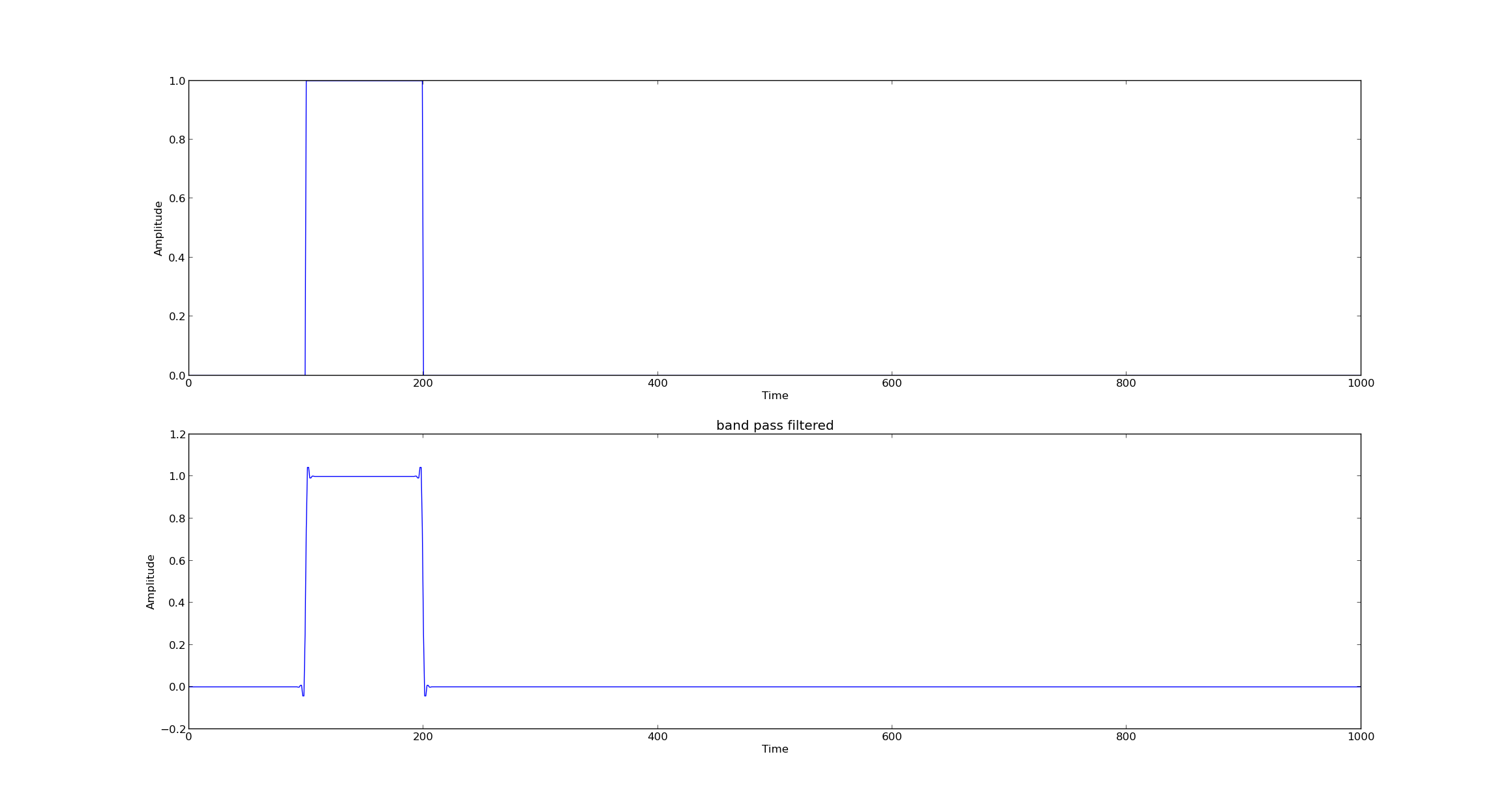
The carrier freuency is 1Khz .The normalized carrier frequency at sampling rate of 5Khz is 0.4. Thus the spectrum of modulated rectangular pulse is centered at 0.4
Thus significant frequency band lies from 0.3 to 0.5.
If we bandpass filter frequencies in this band,we should get a relatively noiseless waveform,which is expected to improve the performance of correlation.
We apply band-pass butter worth filter of order 2 with normalized cutoff frequencies are 0.2 and 0.6.
def butter_bandpass(lowcut, highcut, fs, order=5):
    """ function returns the bandpass butterworth filter coefficients

    Parameters
    -------------
    lowcut,highcut : integer
                     lower and higher cutoff freuencies in Hz

    Fs : Integer
         Samping freuency in Hz

    order : Integer
            Order of butterworth filter

    Returns
    --------
    b,a - numpy-array
          filter coefficients

    """
    nyq = 0.5 * fs
    low = lowcut / nyq
    high = highcut / nyq
    b, a = butter(order, [low,high], btype='bandpass')
    return b, a


def bandpass_filter(data, lowcut, highcut, fs, order,filter_type='butter_worth'):

 """ the function performs bandpass filtering

    Parameters
    -------------
    data : numpy-array
           input signal

    lowcut,highcut : integer
                     lower and higher cutoff freuencies in Hz

    Fs : Integer
         Samping freuency in Hz

    order : Integer
            Order of butterworth filter

    Returns
    --------
    out : numpy-array
          Filtered signal

    """
    global once
    if filter_type=='butter_worth':
        b, a = butter_bandpass(lowcut, highcut, fs, order=order)
        if once==0:
            plt.figure(2)
            plotFrequency(b,a)
            once=1
        y = filtfilt(b, a, data)
        return y
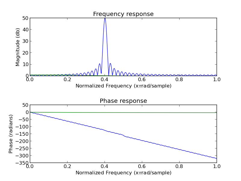
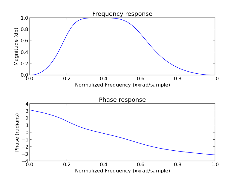
The butter-worth band-pass filter is not a zero phase .It will introduce different phase delay depending of frequency. The.The phase plot of the band pass filter is not linear,
To see the phase delay effects of bandpass butter-worth filter,we consider the case of no noise . we can see that instead of 10,delay is introduced as 12 due to butter-worth filter. However we have a stable singular correlation peak being detected
 *********** Information ************
time delay :  10
Noise : 0.001
SNR 46.9897000434
Correct  0  Incorrect  1000
mean  12.0 Std  0.0
.....
        #introduce delay
        dx=delay(x,tdelay);
        result=numpy.zeros((1,loop));
        for i in range(loop):
            s=dx;

            #add noise
            if varnoise!=0:
                s=addNoise(s,varnoise)

            #normalize signals
            s=s/np.linalg.norm(s);
            x1=x2/np.linalg.norm(x2);
            if carrier!=None:
                unfiltered_signal=s;
                if mode==1:
                    s = bandpass_filter(s, carrier-500, carrier+500, Fs,order,filter_type)
                if mode==2:
                    s = bandpass_filter(s, carrier-750, carrier+750, Fs,order,filter_type)

                filtered_signal=s;
            else:
                unfiltered_signal=s;

            #perform envelope detection
            s=abs(scipy.signal.hilbert(s))
            if mode==1 or mode==2:
                r=numpy.correlate(s,x1,mode="full")

.......
To compensate for that we need to use zero phase filtering techniques like forward backward filtering.
To achieve zero phase the linear filter is applied twice, once forward and once backwards. The combined filter has zero phase.In general forward-backward filtering squares the amplitude response and zeros the phase response if phase of filter is linear.
we see that there are few errors inspire of applying the forward backward algorithm due to distortions introduced by bandpass filtering of high frequency components.Though the mean is closer to actual delay of 10.
 *********** Information ************
time delay :  10
Noise : 0
Correct  0  Incorrect  1000
mean  9.0 Std  0.0
This tells us that we cannot eliminate the effects introduced due to filtering.
we now introduce noise and compare the performance against envelope detection.
 *********** Information ************
time delay :  10
Noise : 0.3
SNR -2.55272505103
Correct  442  Incorrect  558
mean  9.49 Std  0.678159273327
 *********** Envelope Detection ************
time delay :  10
Noise : 0.3
SNR -2.55272505103
Correct  661  Incorrect  339
mean  9.746 Std  0.793400277288
Compared to just envelope detection,we can see that standard deviation has reduced.Thus the neighborhood of estimated TDOA values are reduced,though the mean is shifted away from 10 may be due to the phase delay effects of bandpass filter.
Though band-pass filtering did not lead to a significant improvement due no the noise within the frequency bandwidth .It is essential to keep out unwanted frequency components due to environmental noise and other factors.
Code
The code used in the article can be found in github repository “Github Link”
Files
- TDOA1.py
- TODA2.py - Band Pass Filtering
All the plots included in the article can generated by changing the mode variable in the files