First Order Approximation of DC Motor
10 Apr 2015DC Motor Model
In this article we will look at how to model DC motor and first order model that enables us to quickly predict response of DC motor.
DC Motor
A DC motor is a energy conversion device that converts electric energy to mechanical energy and is a common actuator used in many robotic systems.
A DC motor driven by a voltage and rotates at constant speed that is proportional to the applied voltage and provides rotational torque which when coupled with wheels provides translational motion of the vehicle.
Usually the motor armature has some resistance that limits its ability to accelerate, so the motor will have some delay between the change in input voltage and the resulting change in speed.
DC motor Model
The input of the system is the voltage source $v$ applied to the motor’s armature, while the output is the rotational speed of the shaft $\dot{\theta}$.
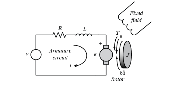
R and L are the armature resistance and inductance.$e$ is called as backemf and is voltage induced in the rotor which results in torque $t$ being produced.
A viscous friction model is generally assumed for DC motor .Where $b\dot{\theta}$ is term which opposed or damps the torque and $b$ is called as damping constant.
Electric Equivalent circut of DC motor
The power supply voltage $v$ is equal to the sum of the voltage drop produced by the current I in the ohmic resistance R of the rotor winding, and the voltage $e$ induced in the rotor
Thus $v = I * R+ e$
The voltage $e$ induced in the rotor is proportional to the angular velocity ω of the rotor
For an armature controlled DC-motor the torque produced by the motor is proportional to only the armature current $i$ by a constant factor $K_{t}$ called motor torque constant.
\[T = K_{t} (i-i_{o})\]$i_{o}$ is the no-load current consumed by the motor to generate torque required to overcome the internal frictions of motor.
The back emf e is voltage induced in the rotor and is proportional to the angular velocity of the shaft by a constant factor $K_{t}$ called the motor/torque constant.
\[e = K_{t} \dot{\theta}\]Ideal Motor
For ideal motor with no losses mechanical power is equal to the electrical power dissipated by the back emf in the armature
$T\omega = e i$ $K_{t} i \omega = K_{e}\omega i$
The motor torque and back emf constants are equal, that is, $K_{t} = K_{e}$
Real Motor
The mechanical power developed by the motor is equal to the sum electrical power given to the motor and the power dissipated
$P_{e} = P{m} + P_{l}$
$P_{e} = v * I$ $P_{m} = T * ω$ $P_{l} =R * I^2 + K_{t}* I_{O} * ω$
The efficiency of the motor is defined as $\eta = \frac{P_{m}}{P_{e}}$
Motor Model
We assume a loss less model in obtaining the first order approximation of the motor model
From Newton’s 2nd law it can be derieved
\[J\ddot{\theta} + b \dot{\theta} = K_{t} i\]where $ J $is the moment of inertia of the rotor $ b $ is the motor viscous friction constant $ K $ electromotive force constant $ i $ is the armature current
Based on Kirchhoff’s voltage law we obtain the equation
\[L \frac{di}{dt} + Ri = V - K_{b}\dot{\theta}\]$R $ electric resistance
$ L $ is electric inductance
$K $ is motor torque constant
$ V $ is input voltage to the motor
$i $ is the input armature current
Applying the Laplace transform, the above modeling equations can be expressed in terms of the Laplace variable s.
\[s(Js + b)\Theta(s) = K_{t}I(s)\] \[(Ls + R)I(s) = V(s) - K_{b}s\Theta(s)\]We arrive at the following open-loop transfer function by eliminating $I(s)$ between the two above equations, where the rotational speed is considered the output and the armature voltage is considered the input.
\[P(s) = \frac {\dot{\Theta}(s)}{V(s)} = \frac{K_{t}}{(Js + b)(Ls + R) + K_{b}K_{t}} \qquad [ \frac{rad/sec}{V}]\]The Block diagram can be expressed as
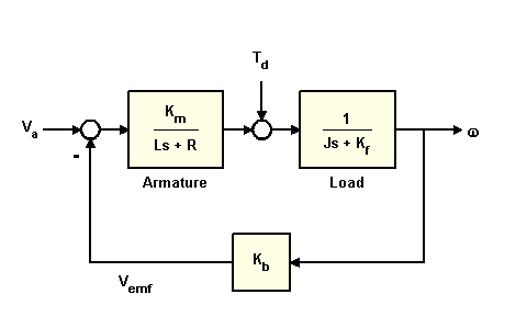 ( In the above diagram Kf=b ,Km=Kb=Kt)
Similarity the transfer function of torque v/s angular velocity can be expressed as
\[\frac {\dot{\Theta}(s)}{\tau(s)} = \frac{-(Ls+R)}{(Js + b)(Ls + R) + K_{b}K_{t}} \qquad\]We assume that ration $\frac{L}{R} \le \frac{J_{m}}{b}$ and we obtain the first order approximation of DC motor as
\[P(s) = \frac {\dot{\Theta}(s)}{V(s)} = \frac{\frac{K_{t}}{R}}{(Js + b)+ \frac{K_{b}K_{t}}{R}} \qquad\] \[P(s) = \frac {\dot{\Theta}(s)}{V(s)} = \frac{\frac{K_{t}}{R}}{Js + (b+ \frac{K_{b}K_{t}}{R})} \qquad\]$\dot{\theta(t)} = v(t) \frac{K_{t}}{RJ}e^{-\frac{(b+ \frac{K_{b}K_{t}}{R})}{J}}$
Thus given an input voltage we can compute the instantaneous angular velocity of the motor .
Example
Let us look at a example of coreless dc motors by portscape
For the present example we use the motor constants from following datasheet
http://www.portescap.com/sites/default/files/26n58_specifications.pdf
J = 6*10-7 kg.cm2
b = 0
Kt = 23.90 mNm/Am
Ke = 2.50 mNm/Am
R = 10 ohms
L = 0.8e-3 h
For ironless motors viscous friction/damping constant $b=0$
Open Loop Response
First we will look at the open loop response of the DC motor . Given input voltage what is the angular velocity of the motor.
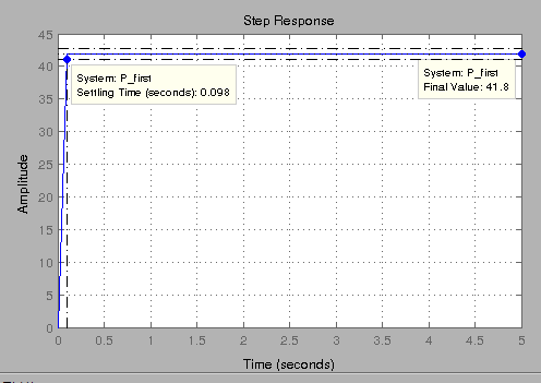
For this we look at the step response of the motor
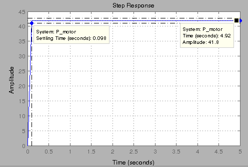
From the plot we see that when 1 Volt is applied to the system the motor can only achieve a maximum speed of 41.8 rad/sec or 399 rpm .Also it takes around 98 msec to reach the desired speed.
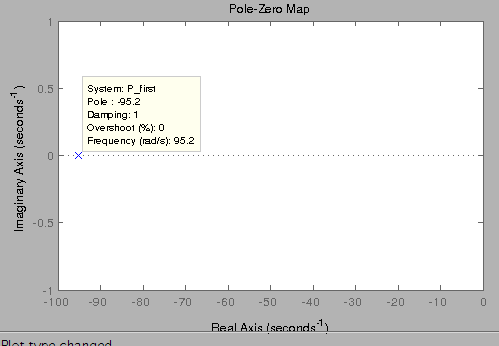
Pole Zero Plot
We can see that the motor model is a second order LTI system,which enables us to predict the characteristics using pole zeros of the transfer function.
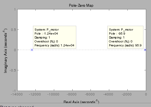
From the the pole zero plot we can see that the open-loop transfer function has two real poles, one at s = -1.24e4 and one at s =-95.9
Since both poles are real, there is no oscillation in the step response (or overshoot) as we have already seen.
First Order Model
We expect the slower of the two poles will dominate the dynamics. That is, the pole at s = -95.9 primarily determines the speed of response of the system and the system behaves similarly to a first-order system.
\[P(s) = \frac {\dot{\Theta}(s)}{V(s)} = \frac{\frac{K_{t}}{R}}{Js + (b+ \frac{K_{b}K_{t}}{R})} \qquad\]Thus the location of the dominant pole is at
$s= \frac{(b+ \frac{K_{b}K_{t}}{R})}{J}$
From the plot we see that when 1 Volt is applied to the system the motor can only achieve a maximum speed of 41.8 rad/sec or 399 rpm .Also it takes around 98 msec to reach the desired speed which is same as the original second order model
We can also see that pole is located at s=-95.2 which agrees with dominant pole of the second order pole which was located at s=-95.9
Now we approximate the motor using first order model and compare the step responses of the model.
With a first-order system, the settling time is equal to
\[T_s = 4 \tau\]where $\tau$ is the time constant which in this case is 0.0105. Therefore, our first-order model has a settling time of 42 ms which is off by order of some ms since the pole is far away from origin.
we can see that a first-order approximation of our motor system is relatively accurate
Information from Step Response
Thus we can predict the motor RPM fairly accurately using the first order system to determine what input voltage to be set to obtain the desired RPM under no load conditions.
The step response gives us idea of voltage vs RPM graph and also the idea about responsiveness of the motor.
\[\dot{\theta(t)} = v(t) \frac{K_{t}}{R*J}*e^{-\frac{(b+ \frac{K_{b}K_{t}}{R})}{J}t}\] \[P(s) = \frac {\dot{\Theta}(s)}{V(s)} = \frac{\frac{K_{t}}{R}}{Js + (b+ \frac{K_{b}K_{t}}{R})} \qquad\]using final value theorem we get
$\dot{\Theta} = V\frac{\frac{K_{t}}{R}}{(b+ \frac{K_{b}K_{t}}{R})}$
This equations helps us compute the angular velocity of motor for any given input voltage.
Let us look at the speed v/s voltage graph
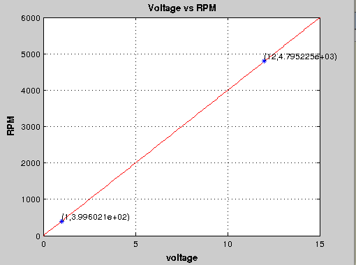
As per the datasheet the rpm at nomial voltage of 12V is 4735rpm which agrees approximately with our estimated of 4975 rpm.We have overestimated the RPM since we have not taken into account the losses in the motor.
Losses in Motor
$v = I * R+ e$ The voltage induced in the motor is not $V$ but $V-RI$
In general It is assumed that at no-load no torque is provided, some torque $\tau_{f}$is required to keep the inertia of the rotor turning and to overcome frictional torques and current draw under is $i_{o}$
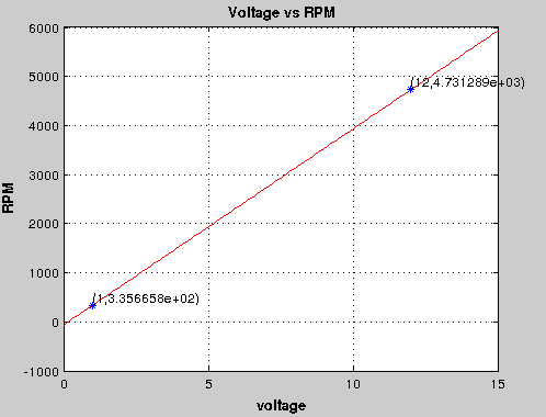
Thus if we take this into account we get estimate of speed at 12V as 4731 rpm which is approximately equal to value of 4735 rpm specified in the datasheet.
This can be verified for different motor models specified in the datasheet
Code
The matlab code can be found at bitbucket repository https://bitbucket.org/snippets/pi19404/55ep